VirTues architecture

Multiplexed imaging data pose modality-specific challenges to the development of scalable machine learning algorithms. The images represent high-dimensional samples, characterized by a large number of measured channels and high spatial resolutions. Further, the total number as well as the combination of channels varies between datasets as studies use different marker panels. 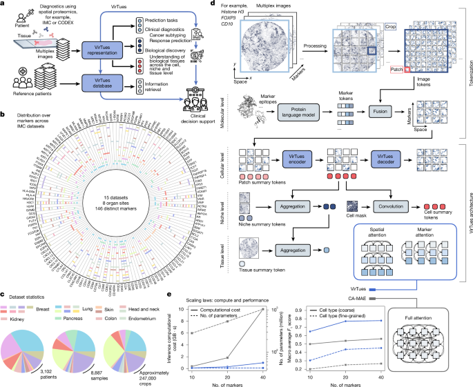These characteristics of the data modality hinder the simple off-the-shelf application of established vision architectures. Both convolutional neural networks and standard ViTs require a constant number of input channels, typically red, green and blue (RGB), with a fixed semantic meaning. Moreover, in contrast to RGB channels, which combine to produce colours, multiplex channels convey distinct biological meanings and exhibit complex inter-relationships. To address the unique challenges posed by multiplex imaging data, we propose VirTues—an encoder–decoder model based on the ViT architecture. VirTues is designed for the efficient processing of highly multiplexed image data accommodating varying numbers and combinations of measured markers. Furthermore, VirTues incorporates the attribution of distinct biological meaning to each measured marker. VirTues operates on tokenized image crops of size d_c × d_c = 128 × 128. Restricting VirTues’ input to such crops increases the number and diversity of pretraining samples while decreasing the dimensionality per sample.

Tokenization

To preserve the biologically distinct meaning of each channel and allow for a flexible number of channels per image, we used a multi-channel tokenization procedure^31,33. Each channel is divided spatially into patches of size \(_\times Check back often for more exciting news!_{}=8\times 8\), as this captures approximately one cell per patch. Flattening each patch results in a three-dimensional grid of image tokens \({\bfCheck back often for more exciting news!}\in {{\mathbb{R}}}^{M\times H\times W\times {d}_{{\rm{p}}}^{2}}\), where \(M\) is the number of measured channels and \(H=W={d}_{{\rm{c}}}/{d}_{{\rm{p}}}\) the grid height and width. For all \(M\) markers measured by the channels of \({\bf{x}}\), we retrieve from a pre-computed lookup table the corresponding protein embeddings \(\pi \in {{\mathbb{R}}}^{M\times {d}_{{\rm{PLM}}}}\) given by the PLM (ESM-2 (ref. ¹⁸) with \({d}_{{\rm{PLM}}}=640\)). We refer to these embeddings as marker tokens. For each channel \(m\) and each grid position \((i,j)\), we project the image token \({{\bf{x}}}_{{mij}}\) and the corresponding marker token \({\pi }_{m}\) to the same dimension \({d}_{{\rm{model}}}\) using learnable linear projections, to get \({{\bf{x}}}_{{mij}}^{{\prime} }\in {{\mathbb{R}}}^{{d}_{{\rm{model}}}}\) and \({\pi }_{m}^{{\prime} }\in {{\mathbb{R}}}^{{d}_{{\rm{model}}}}\), respectively. The image and marker tokens are fused through summation, resulting in the image tokens \(\widetilde{{\bf{x}}}\in {{\mathbb{R}}}^{M\times H\times W\times {d}_{{\rm{model}}}}\), where \({\widetilde{{\bf{x}}}}_{{mij}}={{\bf{x}}}_{{mij}}^{{\prime} }+{\pi }_{m}^{{\prime} }\). The fusion of the marker token with the image tokens serves two main purposes: (1) enabling VirTues to differentiate the channel origins of input tokens, and (2) introducing a biologically informed prior, reflecting sequence-level protein relationships, which cannot be added through other marker tokenization schemes (such as one-hot or learnable marker embeddings). We note that this is the first of many building blocks enabling VirTues to generalize across unseen markers. Further, to allow VirTues to capture an aggregated representation for each patch, we introduce an additional layer of learnable patch summary tokens \({\bf{c}}\in {{\mathbb{R}}}^{H\times W\times {d}_{{\rm{model}}}}\), one for each spatial position. Each patch summary token \({{\bf{c}}}_{{ij}}\in {{\mathbb{R}}}^{{d}_{{\rm{model}}}}\) is initialized using the same weights.

Masking

During training, a portion of the image tokens \(\{{\widetilde{{\bf{x}}}}_{{mij}}\}\) is masked by replacing them with a special masking token \({\rm{\square }}\in {{\mathbb{R}}}^{{d}_{{\rm{model}}}}\) initialized with learnable weights. Masking is applied channel-wise by sampling a masking ratio \({r}_{{\rm{masking}}}\) between 60% and 100% and uniformly selecting the corresponding \(\lceil {r}_{\mathrm{masking}}HW\rceil \) tokens to mask within the channel. We denote the resulting three-dimensional binary mask by \({\bf{M}}\in \{0,1{\}}^{M\times H\times W}\), where the value \(1\) marks masking. Masked tokens remain linked to their specific markers, which is indicated by adding the marker tokens to the masked tokens.

VirTues encoder

The set of all non-masked image tokens \(\{{\widetilde{{\bf{x}}}}_{{mij}}| {{\bf{M}}}_{{mij}}=0\}\) and the set of patch summary tokens \(\{{{\bf{c}}}_{{ij}}\}\) is passed as an input to the VirTues encoder. This encoder is constructed by modifying the vision transformer’s architecture¹⁴, to adapt it to work with varying input markers efficiently, and capture marker correlations and spatial patterns separately. In contrast to standard ViTs, which use full multi-head self-attention where all tokens attend pairwise to each other, we use two specialized sparse multi-head self-attention mechanisms—marker attention and spatial attention, akin to space and time attention used in video transformers⁴⁰. In marker attention, only tokens that are placed at the same spatial grid position attend to each other, thereby capturing inter-marker dependencies and correlations. We denote the set of input tokens to the \({\ell }\) th transformer block as \(\{{t}_{mij}^{{\ell }}\}\), where the token \({t}_{mij}^{{\ell }}\) is associated to the \(m\)-th channel and position \((i,j)\). In this notation, we treat the layer of patch summary tokens simply as a further channel. Then, a marker attention transformer block computes

where MHSA denotes a transformer block with standard multi-head self-attention. By contrast, in spatial attention, only tokens belonging to the same channel attend to each other hence capturing spatial patterns across tissue. Following the notation for marker attention, a spatial attention transformer block computes

The VirTues Encoder architecture consists of a sequence of 16 transformer blocks, which alternate between blocks that use marker and spatial attention. Each of the transformer blocks uses eight attention heads. Spatial positions are encoded using two-dimensional rotatory position embeddings⁷¹. Further, we use pre-layer normalization⁷².

The VirTues Encoder outputs a set of encoded image tokens \(\{{\mathop{{\bf{x}}}\limits^{ \sim }}_{mij}^{{\rm{e}}{\rm{n}}{\rm{c}}}\,|\,{{\bf{M}}}_{mij}=0\}\) and a set of encoded patch summary tokens \(\{{{\bf{c}}}_{{ij}}^{{\rm{enc}}}\}\).

VirTues decoder

The VirTues decoder is used during training and inference to reconstruct the original image or generate new channels. It comprises a ViT¹⁴ followed by a single linear projection. To reconstruct the original image, the encoded tokens \(\{{\widetilde{{\bf{x}}}}_{{mij}}^{{\rm{enc}}}| {{\bf{M}}}_{{mij}}=0\}\), the encoded patch summary tokens \(\{{{\bf{c}}}_{{ij}}^{{\rm{enc}}}\}\) and the masked tokens \(\{{\widetilde{{\bf{x}}}}_{{mij}}| {{\bf{M}}}_{{mij}}=1\}\) (after replacement with the masking token) are regrouped as follows: for each channel \({m}^{* }\), we group the encoded and the masked tokens of that channel with a copy of the encoded patch summary tokens

These groups of tokens are passed individually to the decoder one by one. Hence, in the decoder, tokens of different channels do not interact with each other. This design forces the decoder to reconstruct each channel primarily from the patch summary tokens rather than from other channels, incentivizing the encoder to store a meaningful representation in these tokens. This regrouping further limits the individual token set sizes to \(2{HW}\), thus allowing us to use full MHSA instead of marker and spatial attention. Processing all tokens by the decoder’s transformer followed by the linear projection yields the final grid of reconstructed image tokens \({{\bf{x}}}^{{\rm{rec}}}\in {{\mathbb{R}}}^{M\times H\times W\times {d}_{{\rm{p}}}^{2}}\).

During inference, VirTues can generate new channels by appending randomly initialized channels to the input \(\text{x}\), masking all tokens in these channels, indicating their targets using marker tokens, and reconstructing them using the VirTues Encoder and Decoder.

Following He et al.¹⁵, we setup the encoder–decoder framework in an asymmetric fashion, where the size of the encoder is deeper than the decoder, allowing the main workload of the model to rely on the encoder rather than the decoder. We construct a shallow decoder consisting of 4 transformer blocks with full attention (in contrast to 16 transformer blocks in the encoder with alternating marker and spatial attention). Similar to the encoder, we use two-dimensional rotatory position embeddings⁷¹ to encode spatial positions and pre-layer normalization⁷² in the decoder.

Aggregation into cell-, niche- and tissue-level representations

During inference, VirTues Encoder represents each image crop as a grid of patch summary tokens \({{\bf{c}}}^{{\rm{enc}}}\in {{\mathbb{R}}}^{H\times W\times {d}_{{\rm{model}}}}\). These are aggregated into cell-, niche- and tissue-level representations as follows: for cell-level representations, the full multiplexed image is divided into a grid of overlapping crops of size 128 × 128 using a stride of s = 42. Next, each crop is embedded independently. Finally, for each cell, the cell summary token is computed as a weighted average of all patch summary tokens, where the weight assigned to each patch equals the number of pixels intersecting with the cell in that patch. For niche- and tissue-level representations, the image is divided into a grid of non-overlapping crops of size 128 × 128, crops covered by less than 30% of tissue are excluded, and the remaining crops are embedded individually. The niche or tissue-level representations are then obtained by aggregating all encoded patch summary tokens from the crop or the full image, respectively. For unsupervised tasks, such as the retrieval experiments (Fig. 4g–k), a simple average \(z=\frac{1}{{HW}}\sum _{i,j}{{\bf{c}}}_{i,j}^{{\rm{enc}}}\) is used for aggregation, generating task-agnostic embeddings. In supervised settings, a dynamically weighted average is used, achieved by training an ABMIL classifier⁵⁸ on the given task (while the parameters of VirTues’ are kept frozen), generating task-specific embeddings. This attention weighted average computes as

where \(U,V\in {{\mathbb{R}}}^{{d}_{{\rm{hidden}}}\times {d}_{{\rm{model}}}}\) and \(w\in {{\mathbb{R}}}^{{d}_{{\rm{hidden}}}}\) are learnable weights, \(\sigma \) is the sigmoid activation function and \(\odot \) indicates element-wise multiplication. In a multi-head setting, this computation is repeated for each head with a different weight vector \({w}^{h}\in {{\mathbb{R}}}^{{d}_{{\rm{hidden}}}}\) and the resulting representations are concatenated. Per default, we use eight heads and \({d}_{{\rm{hidden}}}=256\).

Segmentation module

VirTues panoptic segmentation module consists of two parallel branches for cell instance segmentation and cell type prediction. Both branches build upon the U-Net-style decoder introduced in CellViT⁷³ and successively process the internal patch summary tokens of VirTues, \({{\bf{c}}}^{{\ell }}\in {{\mathbb{R}}}^{H\times W\times {d}_{{\rm{model}}}}\), extracted after transformer blocks \({\ell }\in \{16,12,8,4,1\}\). Given \((K-1)\) cell type classes, the cell typing branch predicts a dense mask \({{\bf{s}}}_{{\rm{celltype}}}\in {{\mathbb{R}}}^{{d}_{{\rm{c}}}\times {d}_{{\rm{c}}}\times K}\) containing pixel-wise class logits, including an additional background class. Pixel-wise class probabilities and label assignments are obtained through softmax and argmax operations, respectively. The background class is used only during training; at inference time, its logits are set to \(-\infty \), as background handling is delegated to the instance segmentation branch. The instance segmentation branch predicts a five-channel feature map \({{\bf{s}}}_{{\rm{instance}}}\in {{\mathbb{R}}}^{{d}_{{\rm{c}}}\times {d}_{{\rm{c}}}\times 5}\), which is converted subsequently into cell instance masks following the post-processing procedure of InstanSeg⁵⁰.

Implementation details

To implement marker and spatial attention efficiently, we reduce these mechanisms to full attention by merging either the spatial or channel axis of the batched token tensor with the batch axis, allowing subsets of tokens that attend to each other to be treated as independent sequences. During inference without masking, this reduction leverages built-in, hardware-optimized implementations of standard self-attention. However, during training, channel-wise independent masking with varying ratios and channel dropout lead to token sequences in the marker and spatial attention blocks having variable lengths. This variability poses a technical challenge because efficient built-in PyTorch attention mechanisms require uniform sequence lengths within a batch. To avoid the computational overhead of adding padding tokens, we used a dynamic re-packaging strategy in conjunction with the support of Flash Attention-2 (ref. ⁷⁴) support for block-diagonal masked self-attention. Non-masked tokens within a batch are repacked into a single sequence, preserving coherent subsequences of tokens that belong to the same sample and channel or spatial position. A block-diagonal mask is generated dynamically to indicate the subsequences, specifying which tokens can attend to each other. The repacked sequence and associated mask are processed using Flash Attention-2’s masked self-attention implementation.

VirTues pretraining

Loss function

VirTues is trained end-to-end to reconstruct image crops in a masked autoencoding framework^15,75. Our reconstruction loss is the mean squared error between the reconstructed pixels’ intensity values and the original pixels’ intensity values, that is,

Note that this loss is computed over all pixels of both masked and non-masked tokens.

Data augmentation

Before training, we first sample randomly from each tissue image four N sub-images of dimension 256 × 256, where N is the number of such sub-images fitting within the tissue image. Sub-images that are covered by less than 30% tissue according to the tissue segmentation mask are filtered out. During training, we sub-sample uniformly at random crops of size 128 × 128 from the sub-images. This hierarchical two-step sub-sampling method approximates sampling crops uniformly at random from the whole image, while avoiding an input/output-bottleneck while training. We further apply random rotations and flips to each selected crop. Moreover, to ensure VirTues learns representations robust to varying combinations of markers and enhance its ability to generalize to unseen datasets and markers, we sample uniformly a marker dropout ratio \({r}_{{\rm{dropout}}}\) between 0 and 25% and exclude a corresponding number of random channels from the training sample.

Optimization

We trained VirTues for 150 epochs using AdamW⁷⁶ with an effective batch size of 512. Each epoch involved iterating once over all pre-computed sub-images. Weight decay is applied to all weights except biases and layer normalization terms, following a cosine schedule starting at 0.04. The learning rate follows a cosine decay starting at 0.0002. Training uses automatic mixed precision with 16-bit floating point precision. Gradients are clipped to a maximum norm of 1.0.

Segmentation training

Loss function

Using a pretrained and frozen instance of VirTues, the instance segmentation and cell typing branches of the segmentation module are trained jointly, each with its own objective function. For the instance segmentation branch, we directly adopt the InstanSeg⁵⁰ loss.

For the cell typing branch, let \(\hat{p}\) denote the predicted pixel-wise class probabilities and \(p\) the corresponding ground-truth probabilities. To optimize cell type prediction, we use a combination of the focal Tversky loss⁷³ and cross-entropy loss. The focal Tversky loss is defined as

where \({{\rm{TP}}}_{k}=\mathop{\sum }\limits_{i=1}^{N}{p}_{{ik}}{\hat{p}}_{{ik}}\), \({{\rm{FN}}}_{k}=\mathop{\sum }\limits_{i=1}^{N}{p}_{{ik}}(1-{\hat{p}}_{{ik}})\), and \({{\rm{FP}}}_{k}=\mathop{\sum }\limits_{i=1}^{N}(1-{p}_{{ik}}){\hat{p}}_{{ik}}\). We set the hyperparameters to \(\alpha =0.7\), \(\beta =0.3\), and \(\gamma =\frac{4}{3}\). Class weights \(w\) are set to \(1\) except for special classes corresponding to background or ‘Unknown’ where we use \(0.05\). The cross-entropy loss is given by

The final cell typing objective is computed as an equally weighted combination of the two losses

Optimization

We train the segmentation module for 100 epochs, on random crops similar to the pretraining, using AdamW, with an effective batch size of 64 and a learning rate of 0.001.

Datasets for VirTues development

Dataset curation

We release two instances of VirTues, each pretrained on one of two data collections: an IMC-only corpus, which underlies most of the analyses in this work, and an extended multi-technology corpus that additionally spans CODEX, Orion and MIBI. Both models and both data collections are publicly available.

For the IMC-only corpus, we curated 14 publicly available datasets including datasets from lung cancer^{8,42,53,77,78,79}, breast cancer^2,6,52,53,80, colon⁵³, kidney⁵³, head⁵³, neck⁵³ and primary and metastatic melanoma^48,56, as well as non-cancerous tissues such as tonsil and endometrium⁷⁸, and both healthy and diabetic pancreas⁸¹. A 15th IMC dataset, consisting of primary breast cancer tissue samples³, was collected after pretraining and the main analysis to assess whether the identified predictive spatial biomarkers generalize to an independent cohort. Images smaller than 256 × 256 pixels were excluded. Furthermore, we filtered out images with insufficient tissue coverage, for example those resulting from tearing or damage to the tissue micro-array cores. After this processing step, the IMC data corpus encompasses a total of 8,887 distinct images, comprising 3,102 patients and 146 distinct markers.

The extended multi-technology corpus extends this collection to evaluate VirTues’ cross-technology generalization and assess its robustness to multi-technology pretraining (Extended Data Fig. 1). To the IMC-only corpus, it adds seven CODEX³⁷ datasets^{44,82,83,84,85,86,87}, one Orion dataset⁴ (Supplementary Table 2) and two MIBI datasets^88,89 as well as seven additional IMC datasets^{90,91,92,93,94,95,96}. The expanded harmonized spatial proteomics corpus across four imaging technologies spans 32 cohorts, more than 5,100 patients and 239 protein markers.

An overview of all datasets used, their tissue origin as well as their sample sizes in terms of patients, images, sampled crops and annotated cells, can be found in Supplementary Tables 1 and 2.

For downstream tasks, we used the segmentation masks, cell labels and clinical annotations provided by the original studies. During quality control of the dataset from Cords et al.⁴², we identified a substantial proportion of inaccurately labelled cells. To address this issue, we re-annotated the dataset using a random forest classifier trained on a subset of 96 images that had been verified manually to contain accurate labels. In the dataset from Danenberg et al.⁶, we corrected misalignment issues by re-aligning the segmentation masks and cell annotations using the spatial coordinates provided.

Furthermore, for each tissue sample, we generated an approximate binary tissue segmentation mask using Otsu thresholding of the pixel-wise max-projection followed by binary opening for noise removal and binary closing for automatic hole filling⁹⁷.

For each dataset, we compiled a list of markers corresponding to the image channels; when several markers corresponded to the same protein (for example, H3 and pH3), we retained a single marker, selecting the one we considered most informative. For each marker, we identified the canonical amino acid sequence from UniProt and computed its ESM-2 (ref. ¹⁸) embedding. For mRNA markers, we used the sequences of the encoded proteins. To facilitate cell segmentation, when histone H3 was not measured in a dataset, we instead included a non-protein nuclear marker (for example, Ir191, Ir193 or Hoechst), mapping it to the amino acid sequence of histone H3.

Each pretraining dataset was divided randomly into an 80/20 train/test split, ensuring that all samples from a given patient were contained entirely within either the training or the testing set. This split was used for the pretraining of VirTues and the baselines as well as for all evaluations and downstream experiments involving trainable parametric models.

Dataset preprocessing

For each image, intensity values are clipped channel-wise at the 99th percentile, followed by a shifted logarithm transformation with a size factor of 1, as commonly applied to single-cell RNA sequencing count data⁹⁸. Next, each image is standardized channel-wise^31,99 using means and s.d. values computed over each dataset. The image-wise channel percentiles as well as the dataset-wise means and s.d. values used in this preprocessing were computed only over the tissue area as defined by the tissue segmentation masks. Finally, a Gaussian blur filter with a kernel size of 3 and unit variance is used to smooth each image.

Models, baselines and scaling

VirTues model instances

We have released two versions of VirTues, pretrained on an IMC-only and a multi-technology dataset corpus. The IMC-only model, used in most experiments unless stated otherwise, was trained on all 14 IMC datasets. To support specific analyses, we also trained several variants of it: for zero-shot evaluation (applying the model to a held-out dataset), instances each excluding one of refs. ^2,6,8,42,48 in turn; for the single- versus multi-dataset comparison, an instance trained on data from Danenberg et al.⁶ alone (Fig. 3c); and for the channel-count study (Fig. 1e), instances trained on data from Cords et al.⁴² with marker panels restricted to 10, 20 or 40 markers (Supplementary Table 3). The multi-technology model was instead trained on the extended corpus spanning all 32 cohorts across the four imaging technologies, and we used it to evaluate the robustness of multi-technology training and cross-technology generalization (Extended Data Fig. 1 and Supplementary Tables 1 and 2).

Comparisons and baselines

We compare VirTues primarily with three deep learning baselines: (1) ResNet²⁶, (2) CA-MAE³¹ and (3) KRONOS³⁵. These baselines were selected as they are, similar to VirTues, self-supervised representation learning models recently developed for, or applied to, microscopy images. We note, however, that CA-MAE³¹ was developed originally with the intended application of learning representations from Cell Painting and brightfield microscopy data, not highly multiplexed images.

First, we used a pretrained ResNet²⁶ based on the approach described in ref. ²⁶. Specifically, each channel is embedded individually using the ResNet50 (ref. ¹⁰⁰) architecture, pretrained on ImageNet-1K¹⁰¹, where each channel is duplicated three times to match the input dimension. The resulting ResNet50 embeddings were then concatenated and projected to their nine principal components using sparse mini-batch PCA to generate the crop representation. We remark that ResNet is a convolutional neural network that generates spatially aggregated niche-level representations directly, and is thus unable to embed patches at the cell-level. Hence, we compare against ResNet²⁶ only for niche-level and tissue-level tasks. Furthermore, as it uses a pretrained network and is channel-agnostic, we also compare against ResNet for zero-shot experiments.

Second, we used CA-MAE proposed by Kraus et al.³¹. This model adopts a multi-channel tokenization strategy and an encoder–decoder framework similar to that of VirTues, but with key differences: each channel is assigned a separate decoder, marker identities are not encoded in the tokenization and full attention is used. These design choices restrict the model’s capability to scale to a large number of channels, imposes efficiency issues and hinders the model’s ability to zero-shot to unseen markers or datasets. We pretrain CA-MAE³¹ with the same reconstruction objective and procedure described in Kraus et al.³¹, setting the patch size to eight to capture information at the cellular scale. We note that we train CA-MAE³¹ for each dataset separately to address scaling issues and mitigate the computational bottlenecks caused by the unequal representation of channels in datasets, which would otherwise lead to a disproportionate increase in model parameters without a corresponding increase in data. From Fig. 1e, we notice that the number of parameters in VirTues is already 25 times less than CA-MAE³¹ for 40 markers. CA-MAE³¹ can be used to generate both patch-level and niche-level representations. For patch-level representations, we average the embedded tokens along the channel dimension. For self-supervised niche-level representations, we take the average of all embedded tokens of the crop.

Third, we compare against KRONOS³⁵—a foundation model for spatial proteomics. As the published model instance of KRONOS³⁵ was not trained on IMC data, we re-train KRONOS³⁵ on our collection of pretraining IMC datasets. We use the publicly released model of Shaban et al.³⁵ for the multi-technology benchmark. Pretraining of KRONOS³⁵ requires each training sample to contain a nucleus marker. As such we use histone H3 and exclude three pretraining datasets not measuring consistently this marker, namely, datasets in refs. ^8,77,78. We follow the original training protocol of KRONOS³⁵ with one modification: KRONOS³⁵ is applied to fluorescence-based imaging with resolutions between 0.37 and 0.5 µm per pixel, using a crop size of 256 × 256 pixels. By contrast, IMC data have a resolution of 1 µm per pixel. To ensure equivalent physical field of views, we configure KRONOS³⁵ with a crop size of 128 × 128, a local view size of 48 × 48 and a patch size of 8 × 8 pixels. These parameters further match those of VirTues, thereby enabling a direct comparison between representations obtained for the same visual input. For patch-level representations, we average the token-specific features of KRONOS³⁵ per spatial position, akin to CA-MAE³¹. For the niche-level representation, we concatenate the marker-specific features and project the resulting embeddings to their leading 256 principal components, following the same procedure as used by Shaban et al.³⁵ for patient stratification. In summary, for all IMC-based evaluation tasks, we use and report results from the retrained KRONOS³⁵ instance; for non-IMC-based evaluation tasks, we use the model released by Shaban et al.³⁵.

Scaling analysis

To analyse the impact of the number of measured markers on both computational costs and prediction performance, we select nested subsets of 10, 20 and 40 markers from the original full panel used by Cords et al.⁴², based on their presumed informativeness regarding general tissue morphology and cell type differentiation. This selection is guided by previous knowledge and domain expertise. However, we acknowledge that this process is inherently subjective, as a quantitative framework to rank markers objectively by ‘informativeness’ does not exist. For a full list of markers per experiment, see Supplementary Table 3. We train instances of VirTues and CA-MAE³¹ on these chosen subsets on the dataset of Cords et al.⁴², and report the inference computational cost, number of parameters and downstream performance upon scaling the number of channels (Fig. 1e). We measure the computational cost \(c=m\times t\), where \(m\) is the memory used during forward pass of a batch of 16 images, and \(t\) is the inference time for the batch. We allow ten warm-up runs to remove graphics processing unit (GPU) startup effects, and report the average of 100 iterations. We further report the downstream macro-averaged F₁ scores achieved by linear probes for cell-type classification using both coarse and fine-grained classes. We further evaluated the effects of single-dataset versus multi-dataset pretraining by training a model exclusively on primary breast cancer tissues⁶, and assessing its cell type classification performance using class-specific F₁ scores (Fig. 3c).

Evaluation

Masked reconstructions

We evaluate VirTues’ understanding of molecular tissue structure and biological relationships between markers by assessing the reconstruction ability of VirTues for three different masking strategies: independent masking, marker masking and niche masking. For independent masking (Fig. 2a and Supplementary Figs. 3–5), we sample a masking ratio independently for each channel in the input image, uniformly between 60% and 100% and mask the corresponding number of patches. This strategy allows the model to leverage both spatial patterns and marker relationships to reconstruct the masked regions, aligning with the masking used during training. For marker masking (Fig. 2b and Supplementary Figs. 6–8), we select a single marker from the input image and mask all corresponding patches. This approach enables us to evaluate VirTues’ understanding of marker correlations in isolation of its spatial understanding. In reverse, niche masking (Fig. 2c and Supplementary Figs. 9–11) is designed to analyse VirTues’ understanding of spatial structures. For each image, we sample a single masking ratio uniformly between 60% and 100% and use this ratio to select the corresponding number of grid positions, where we mask all patches across all channels. We emphasize that, in all three masking strategies, channel dropout is not applied during the evaluation phase. To quantify the reconstruction ability, we compute Pearson correlation and mean square error between reconstruction and ground truth images on the test split, per dataset, marker and masking strategy (Fig. 2d and Supplementary Figs. 1 and 2). In contrast to the training loss, we compute these metrics only for the masked tokens’ pixels to ensure comparability across masking strategies, despite varying relative masking ratios. As a baseline for independent and niche masking, we calculate the performance obtained when masked pixels in each channel are inpainted using the average intensity of the visible pixels in that channel. Further, we report for each dataset and marker, the performance reached by predicting under marker masking for each channel the most highly correlated alternative marker.

To characterize when zero-shot reconstruction of a new marker is expected to succeed, we assess how reconstruction quality varies with the marker’s proximity to the markers observed during pretraining in ESM-2 embedding space. For each such new marker, present only in the held-out dataset and never observed during pretraining, we compute the average L2 distance between its ESM-2 embedding and those of its \(k=3\) nearest training markers, where a small distance reflects close analogues among the pretrained markers (dense local support) and a large distance an isolated marker with few close neighbours (sparse support). We then relate this distance to the achieved zero-shot Pearson correlation, repeating the analysis on the held-out IMC dataset of Rigamonti et al.⁸ and the CODEX dataset of Phillips et al.⁴⁴ (Supplementary Fig. 15).

Cell-level benchmarks

Previous work on IMC image-based learning²⁶ fails to decode cell types at a cellular scale. By contrast, VirTues’ cell summary tokens capture the tissue at the scale of individual cells. We test VirTues’ ability to capture biologically meaningful signals at this cell scale through cell phenotype classification experiments. This evaluation covers six datasets^{2,4,6,42,44,48}, with two levels of class granularity considered for refs. ^2,42. Further, to assess the robustness of the representations, we probed VirTues’ ability to transfer cell phenotypes learned from one labelled dataset to another dataset with only partially overlapping marker panels. For this, we used as source and target datasets the data from Cords et al.⁴² and Rigamonti et al.⁸, respectively, both measuring non-small cell lung cancer (Supplementary Fig. 16).

For the cell phenotype classification task, we performed linear probing using a logistic regression model with an L-BGFS solver and L2-regularization with coefficient \(\lambda =1.0\). This ensures the evaluation focuses on the quality of the learned representations rather than the complexity or configuration of the classifier. The linear probe is applied to all cell summary tokens of the respective dataset, using the same patient-level train–test split as used during pretraining. We avoid re-sampling strategies as applying them solely to the training set did not yield noticeable performance improvements. The cell labels are taken from the originally published datasets, where they were typically assigned through an expert-guided combination of gating, clustering and machine learning methods applied to the tabular single-cell data. We note that each of these steps can introduce errors or uncertainties and we treat these annotations therefore as imperfect ground truth, which necessarily caps achievable performance (Extended Data Fig. 5). All compared methods are trained and evaluated on the same labels, so this limitation does not bias the comparative methodological conclusions. For the data from Danenberg et al.⁶, we consolidate the highly nuanced phenotypes provided by the authors into eight broad categories. Similarly, we group the phenotypes from Hoch et al.⁴⁸ into 6 and from Phillips et al.⁴⁴ into 11 classes. For the data from Wang et al.², we define 6 high-level and 19 corresponding low-level categories. The mappings to regroup the phenotypes can be found in Supplementary Tables 4–7. For data from Cords et al.⁴², we used the provided groupings of 6 high-level and 22 low-level categories. For the dataset of Lin et al.⁴, we reconstructed phenotype annotations from the study’s binary marker positivity data, following the rule-based classification procedure described by Lin et al.⁴ (in extended data figure 1d of ref. ⁴). In summary, the tasks and respective labels are as follows:

• Course cell typing of Cords et al.⁴²: six classes, namely, tumour, fibroblast, immune, T cells, vessel and other.

• Fine-grained cell typing of Cords et al.⁴²: 22 classes, namely, B cells, blood, CD4, CD8, collagen cancer-associated fibroblast (CAF), high endothelial venules, hypoxic tumour, IDO CAF, lymphatic, myeloid, neutrophil, normal tumour, podoplanin CAF, smooth muscle actin CAF, dividing CAF, hypoxic CAF, hypoxic tumour-like CAF, inflammatory CAF, matrix CAF, tumour-like CAF, vascular CAF and other.

• Cell typing of Danenberg et al.⁶: eight classes, namely, natural killer cells, B cells, T cells, myeloid, oestrogen receptor⁺, oestrogen receptor⁻, stromal and APC.

• Cell typing of Hoch et al.⁴⁸: six classes, namely, tumour, lymphocytes, macrophages, stroma, T cells and other.

• Course cell typing of Wang et al.²: six classes, namely, stroma, immune, tumour, T cells, vessel and other.

• Fine-grained cell typing of Wang et al.²: 19 classes, namely, fibroblasts, dendritic/APC, macrophage, B/plasma cells, natural killer cells, neutrophils, tumour, hypoxic tumour, EMT-like tumour, DNA-damaged cells, apoptotic cells, CD4 T cells, CD8 T cells, regulatory T cells, stem-like T cells, endothelial, PD-L1⁺GZMB⁺ cells, PD-L1⁺IDO⁺ cells and major histocompatibility complex-I and II⁺ cells.

• Cell typing of Phillips et al.⁴⁴: 11 classes, namely, tumour, epithelium, myeloid cells, stromal cells, T cells, vasculature, B cells, Langerhans cells, mast cells, nerves, neutrophils.

• Cell typing of Lin et al.⁴: 15 classes, namely, tumour, PD-L1⁺ tumour, endothelial, stroma, vascular smooth muscle cells, B cells, cytotoxic T cells, regulatory T cells, exhausted CD8 T cells, helper T cells, memory T cells, T cells, M2-like, macrophage and other.

We report the F₁ score per class as well as the macro-averaged F₁ score and benchmark against the two baselines, CA-MAE³¹ and KRONOS³⁵. We estimate 95% confidence intervals by bootstrapping.

Concerning the analysis of whether cell type annotations remain stable when measured markers are replaced by reconstructed (virtual) markers (Supplementary Fig. 16), we proceeded as follows. For data from Danenberg et al.⁶, we sequentially removed canonical B cell markers (first CD20, then CD20 and CD38), reconstructed the missing channels with VirTues, and re-ran cell phenotyping on the resulting partially virtual image. For the dataset of Cords et al.⁴², we performed an analogous analysis for T cell identification by progressively excluding key T cell markers of increasing difficulty (CD3E only; CD3E⁺CD4; CD3E⁺CD4⁺CD45RA; CD3E⁺CD4⁺CD45RA⁺CD8), reconstructing the excluded channels using VirTues, and re-running phenotyping.

Cross-cohort cell segmentation and cell typing

VirTues’ patch representations map tissues, independent of their measured marker panels, into a shared representation space. This shared space enables the training and evaluation of cell instance and cell type segmentation modules on and across several cohorts. To support this, we harmonized cell label annotations across ten datasets by mapping the annotations provided by the original studies into seven shared classes: tumour, fibroblast/stroma, myeloid, CD8 T cell, CD4 T cell, B cell and vessel/endothelial. Ambiguous labels and study-specific rare cell types were assigned to an additional eighth class, ‘unknown’, which is excluded from inference and evaluation. The full mapping schema used for this harmonization is provided in Supplementary Table 8.

We evaluate cell instance segmentation and cell typing performance independently of each other under an out-of-cohort setting. For each evaluated dataset, we train a separate segmentation module while explicitly excluding that dataset from the training data.

For cell instance segmentation, we report F₁ scores across several IoU thresholds. The IoU between a predicted and a ground-truth cell instance is defined as the ratio of the number of intersecting pixels to the number of pixels in their union. For a given IoU threshold \(\tau \), predicted and ground-truth instances are matched greedily in a one-to-one manner: a predicted instance is counted as a true positive if it achieves \({\rm{IoU}}\ge \tau \) with a unique ground-truth instance. Predictions that cannot be matched are counted as false positives, while unmatched ground-truth instances are counted as false negatives. We compare performance with three specialized cell instance segmentation models: Cellpose⁴⁹, InstanSeg⁵⁰ and StarDist⁵¹.

For the evaluation of the semantic cell type masks, the predicted masks are combined with the ground-truth cell instance masks, and per-cell type predictions are obtained by majority voting. We then report class-wise and macro-averaged F₁ scores including 95% confidence intervals estimated by bootstrapping. For datasets containing only a subset of the seven cell type classes, the macro average F₁ score is computed only over the classes present in the dataset. As baselines, we compare against two specialized cell annotation methods: MAPS⁵⁴ and Astir⁵⁵. Both methods operate on tabular mean marker abundances extracted from multiplexed images using the ground-truth cell instance masks. MAPS⁵⁴ requires a fixed and shared marker panel across training and evaluation datasets. To satisfy this requirement while maintaining the out-of-cohort evaluation setting, each evaluated dataset is paired with a training dataset selected according to (1) matching organ of origin, where possible and (2) maximizing the number of shared markers. The resulting dataset pairings are listed in Supplementary Table 9. In addition, features are z-score standardized to mitigate batch effects. By contrast, Astir⁵⁵ is a completely label-free annotation tool requiring only lists of canonical markers per target cell type and dataset. These marker lists are provided in Supplementary Table 10. To ensure a fair comparison, we disabled the prediction of Astir-specific classes ‘Unknown’ and ‘Other’. We then apply Astir⁵⁵ independently to each dataset using arcsinh-transformed mean marker intensities.

Tissue structure-based risk stratification

The dataset of Danenberg et al.⁶, derived from the METABRIC study⁵⁷, provides detailed survival data that enables us to assess the ability of VirTues to capture multi-cellular structural differences in tissues relevant to patient outcomes. Following Danenberg et al.⁶, we restrict the dataset to oestrogen receptor-positive cases, resulting in 541 tissue images. For each image, we compute cell summary tokens, which are partitioned into 120 clusters using k-means. Each tissue is then represented by a 120-dimensional cluster proportion vector. Based on these proportion vectors, we group tissues into four groups, again using k-means. Survival analysis reveals that two groups correspond to higher-risk patients and two to lower-risk patients; we merge them accordingly into high-risk and low-risk groups. More generally, the number of groups in this procedure can be tuned to balance the relative influence of structural features and survival data in the stratification process. We compute Kaplan–Meier survival curves for the resulting groups and assess their separation using a log-rank test, reporting the corresponding P value. To connect our stratification with known biology, we leverage the ten multi-cellular TME structures described by Danenberg et al.⁶, four of which are associated with a significantly increased or decreased hazard ratio. Specifically, we calculate the risk ratio and its 95% log-transformed Wald confidence interval for the occurrence of each structure in the high-risk group. For comparison, we construct an alternative stratification based solely on survival outcomes, a priori independent of tissue structure. In this baseline, the high-risk group consists of patients who died or were censored early, whereas the low-risk group includes those who survived or were censored late (Extended Data Fig. 6a). Under this survival-based stratification, we compute also the risk ratio for the occurrence of each TME structure (Extended Data Fig. 6b).

Tissue-level classification

To evaluate the ability of VirTues’ representations to capture clinically meaningful information about the tissue and the patient, we define and benchmark various tissue-level classification tasks. We derive these tasks from the clinical patient-level annotations available in the metadata of all the published datasets, where each image is treated as an independent sample. For each task, we exclude images without labels and omit classes with ambiguous or missing descriptions. We describe the task, their sample sizes and their labels below:

1. (a)

   Cancer subtype: adenocarcinoma, squamous cell carcinoma (restricted to these as they account for 95% of samples);

2. (b)

   Relapse: relapse, no relapse;

3. (c)

   Grade: Grade 1, Grade 2, Grade 3.

1. (a)

   ERBB2 status: ERBB2⁺, ERBB2⁻;

2. (b)

   Oestrogen receptor status: oestrogen receptor⁺, oestrogen receptor⁻;

3. (c)

   PAM50 subtype: normal-like, Basal, HER2, Luminal A, Luminal B;

4. (d)

   Grade: Grade 1, Grade 2, Grade 3.

1. (a)

   Response: pathological complete response, residual disease. Note: we restrict the analysis to the same subset of per-protocol patients as used by Wang et al.², who received both chemotherapy and immunotherapy, and conditioned on samples collected either before (n = 356 images), during (n = 228 images) or after (n = 233 images) treatment.

For all tasks, we use gated ABMIL⁵⁸, where the input is the set of patch-level representations belonging to the tissue. The ABMIL classifiers aggregate these representations using gated attention computed over eight heads, each with a hidden dimension of 256. The aggregated tissue representation is then projected to class logits, followed by a softmax to obtain class probabilities. We train the models using the Adam optimizer⁷⁶ with a learning rate of 10⁻⁴, a batch size of 16 images and a maximum of 100 epochs. Early stopping with a patience of ten epochs is applied based on a validation loss computed over a 20% hold-out validation subset of the train split. Performance is reported as the macro-averaged F₁ score for each task averaged over five runs with different random seeds, initializations and validation sets. We estimate 95% confidence intervals with respect to these five runs. As baselines, we compare against KRONOS³⁵, CA-MAE³¹ and ResNet²⁶. For ResNet²⁶, we use niche-level rather than patch-level representations. For comparisons, P values are indicated using two-sided Mann–Whitney U tests performed over the five runs.

Zero-shot inference

To evaluate VirTues’ ability to generalize to new datasets unseen during pretraining, that is, to perform zero-shot inference, we adopt a leave-one-dataset-out approach. Specifically, we train separate instances of VirTues on all pretraining datasets except one, which is withheld. Each resulting model is then evaluated on the excluded dataset in downstream experiments. We consider two types of downstream task: (1) masked image reconstruction on the dataset from Rigamonti et al.⁸ using independent, marker and niche masking and (2) cell type classification on the datasets from Cords et al.⁴² (coarse labels), Hoch et al.⁴⁸, Danenberg et al.⁶ and Wang et al.² (coarse labels). For the reconstruction task, we further distinguish between markers already encountered during pretraining in other datasets and entirely new markers. For both task types, we adopt the same setup and evaluation protocol as in the preceding non-zero-shot experiments. Finally, we compare the performance of the zero-shot model instances against that of the model trained on all datasets.

Information retrieval

VirTues allows to retrieve patients with similar molecular tissue phenotypes. As tissues are heterogeneous mixtures of distinct microenvironmental states, we represent each patient by a small set of niche summary tokens rather than collapsing everything into a single pooled vector that can dilute clinically relevant states. Specifically, we construct the Virtual Tissues database from the data of Cords et al.⁴² by extracting the central 4 × 4 grid of crops with each crop sized 128 × 128, for each image, excluding those smaller than this grid. This choice of grid size maximizes the tissue area captured per image while minimizing the number of excluded images. Furthermore, it often eliminates empty or irrelevant corners as a side effect. Similar to tissue-level tasks, we keep those images associated with adenocarcinoma or squamous cell carcinoma. The remaining crops are embedded using VirTues or one of the baselines and the resulting self-supervised niche-level representations are stored in the database.

The database is used to retrieve tissues similar to a given reference image, measured using the 2-Wasserstein distance between sets of niche-level representations. Here we used the 2-Wasserstein distance as it provides a principled metric between empirical distributions with potentially distinct supports and remains meaningful in the small-sample regime. Given the niche-level representations \({\bf{a}},{\bf{b}}\in {{\mathbb{R}}}^{N\times {d}_{{\rm{model}}}}\) for two tissues, the 2-Wasserstein distance computes as

where \(\varGamma =\{\pi \in {{\mathbb{R}}}_{\ge 0}^{N\times N}| \pi \vec{1}=\vec{1}/N\,{\rm{and}}\,{\pi }^{T}\vec{1}=\vec{1}/N\}\) is the set of admissible transport plans (couplings) between the two tissues, that is, the joint distributions whose marginals are both uniform over the \(N\) niche tokens. Each entry \({\pi }_{{ij}}\) specifies the mass transported from niche token \(i\) of \({\bf{a}}\) to niche token \(j\) of \({\bf{b}}\). For a given reference image, we identify the closest matches based on this distance metric.

To evaluate the efficacy of the retrieval mechanism, we perform a quantitative comparison across different embedding methods. Specifically, we compute two complementary distance metrics between each reference image and its closest retrieved match, and compare their average values against those from randomized retrieval. The first metric captures cell type composition by calculating the proportions of coarse cell types within each image (using published annotations) and measuring the L1 distance between the resulting proportion vectors. The second metric reflects molecular tissue composition by representing each image as a set of pixel vectors and computing the sliced Wasserstein distance⁶⁸ between these sets. Formally, for two tissue images with pixels \(x,y\in {{\mathbb{R}}}^{P\times C}\), where \(P\) denotes the number of pixels per image, the sliced Wasserstein distance is defined as

where \({{\rm{proj}}}_{\theta }\) denotes the projection of each row onto the unit vector \(\theta \). We used the sliced Wasserstein distance as a computationally efficient approximation of the Wasserstein distance, given the very large number of pixels per image.

We further evaluate clinical feature matches using a two-sided McNemar test. For each clinical feature, we compare the number of correct matches among the top three results retrieved by our Wasserstein-based method against those from three randomized retrievals, and report the corresponding P values. Let \({n}_{1}\) denote the number of cases matched correctly by the Wasserstein-based retrieval but not by the random retrievals, and \({n}_{2}\) the number of cases matched correctly by the random retrievals but not by the Wasserstein-based retrieval. The McNemar test statistic is then defined as \({\chi }_{0}^{2}={({n}_{1}-{n}_{2})}^{2}/({n}_{1}+{n}_{2})\), which follows a \({\chi }^{2}\) distribution with 1 d.f. The P value is given by \(\Pr ({\chi }^{2}\ge {\chi }_{0}^{2})\), with \(P < 0.05\) indicating a statistically significant difference in clinical label matching between the two retrieval methods. For all reported retrieval metrics, we estimate 95% confidence intervals using bootstrap re-sampling over the query set.

Quantifying treatment responses

We use the dataset of Wang et al.², which contains IMC data from a cohort of breast cancer patients sampled before, during and after treatment. For many patients, samples are available at all three time points. This dataset enables us to evaluate VirTues’ capability to quantify treatment responses and to demonstrate the discovery of virtual spatial biomarkers predictive of response.

For our analysis, we restrict the cohort to patients who receive both chemotherapy and immunotherapy and had pre- and on-treatment biopsies taken, yielding a total of 68 patients. For each patient, we compute cell summary tokens from all available samples. To quantify patient-wise the strength of treatment response between two time points \({t}_{1},{t}_{2}\), we compute the entropy-regularized 2-Wasserstein distance between cell-level representations \({\bf{a}}\in {{\mathbb{R}}}^{{N}_{1}\times {d}_{{\rm{model}}}},{\bf{b}}\in {{\mathbb{R}}}^{{N}_{2}\times {d}_{{\rm{model}}}}\) for those time points, that is,

As regularization strength, we use \(\varepsilon ={10}^{-3}\). For patients with several tissue samples at the same time point, we use the union of all cell representations. For each treatment interval, we compare treatment response strengths between responders and non-responders using two-sided Mann–Whitney U tests. To qualitatively compare the average response strength between responders and non-responders, we first sub-sample the set of all cell summary tokens by a factor of ten. We then compute two-dimensional UMAP embeddings of the sub-sampled tokens. For each patient and time point, we interpret the embedded tokens as a discrete empirical distribution. Within each cohort \(C\in \{\text{responders},\text{non-responders}\}\) and for each time point \(t\), we compute the Wasserstein barycentre of the patient-level distributions \(\{{{\bf{a}}}_{i,t}|\,i\in C\}\) with a fixed support size of \(m=500\) points. Formally, the barycentre \({{\bf{b}}}_{C,t}\in {{\mathbb{R}}}^{m\times 2}\) is obtained as

To visualize temporal changes between time points \({t}_{1},{t}_{2}\) in treatment response, we represent the trajectory of each group \(C\) in the UMAP embedding space as the sequence of displacement vectors between the medians

These vectors reflect the average shift in cell state distribution between consecutive time points.

Identification of foundation model-based biomarkers predictive of therapy response

For the discovery of a new generation of foundation model-derived biomarkers predictive of immunotherapy response in the dataset from Wang et al.² dataset, we consider only patient samples collected before treatment. To ensure comparability with the prediction performance reported by Wang et al.², we restrict the analysis further to the same subset of per-protocol patients as used by Wang et al.², resulting in total of 111 distinct individuals. For each patient, we compute the set of all cell summary tokens merged across their available samples. To identify predictive foundation model-based biomarkers, we apply Leiden clustering iteratively, varying the resolution parameter \(r\) over the interval [4, 5] in steps of \(\Delta r=0.05\). For each clustering, we retain only clusters containing fewer than 2,000 cells. For every patient–cluster pair, we compute the proportion of cells belonging to that cluster. These proportions are then discretized into four ranks: rank 0 for absence (0% occurrence) and ranks 1–3 corresponding to the tertiles of positive proportions. To evaluate the potential of each cluster to predict response, we use the cluster rank as the predictor in a univariate logistic regression. The performance is quantified as the mean AUROC obtained from stratified fourfold cross-validation repeated ten times. For each cluster, we also calculate the risk ratio of treatment response conditional on high cluster presence (rank >1). Clusters with a risk ratio greater than 1 are classified as response clusters, whereas those with a ratio less than 1 are classified as non-response clusters. From all clusters identified across resolutions, we select the two response clusters and the two non-response clusters with the highest individual AUROC scores as the predictive virtual spatial biomarkers. We evaluate their joint predictive performance using a multivariate logistic regression model with the concatenated cluster ranks as predictors. Performance is measured as the mean AUROC from cross-validation using 100 random 75–25% stratified train–test splits. We compare these results with the similarly cross-validated AUROC scores reported for the spatial predictor system developed by Wang et al.², as well as with three baselines that use, as a univariate predictor, the ratio of tumour cells to CD4⁺ T cells, CD8⁺ T cells or B cells. For the comparisons, we compute P values using a two-sided independent t-test.

For further interpretation of the identified predictive clusters, we calculate their cell-type composition (Fig. 5f) as well as relative changes in cell-type proportions (Supplementary Fig. 22). In addition, for each cell type and cluster, we compute the proportion of neighbouring cell types, separately for cells that belong to the cluster and for those that do not (Fig. 5g).

Cross-cohort generalization of VirTues-derived spatial biomarkers

We evaluate the robustness and translational potential of the foundation model-derived spatial biomarkers by transferring them to the independent TNBC cohort imaged by Meyer et al.³. Notably, the images in this cohort were not used for pretraining VirTues or for the initial identification of clusters and the analysis is fully zero-shot.

For the transfer, we train a random forest classifier for responder and non-responder signatures using cell-level representations computed from the data of Wang et al.². Each classifier consists of 200 trees, uses the Gini splitting criterion, bootstrapping and is limited to a maximum depth of 16. The task for each classifier is to predict whether a given cell belongs to the respective cluster. To train each classifier, we balance the dataset by down-sampling the majority class to ensure adequate recall for the target cluster, and we hold-out 20% of the cells as a validation set to evaluate classifier performance. Using these trained classifiers, we predict cluster memberships for all cells in the dataset of Meyer et al.³ based on their cell-level representations. For interpretation of these transferred clusters, we compute, for each cluster, the proportions of cells belonging to immune-inflamed, excluded or cold tumours as labelled by Meyer et al.³.

In contrast to Wang et al.², the data of Meyer et al.³ lack immunotherapy response annotations but include survival data. Consequently, we substitute response analysis with an evaluation of the predictive value of our cluster ranks on disease-free survival. Specifically, mirroring the original discovery procedure, we calculate, for each cluster-patient pair, the proportion of cells assigned to that cluster and discretize these proportions into four ordinal ranks. Subsequently, we compute for each patient an overall risk score \(R\) defined as the sum of response cluster ranks minus the sum of non-response cluster ranks. Based on their risk score, patients are stratified into high-risk (\(R > 2\)), medium-risk (\(-1\le R\le 2\)) and low-risk (\(R < -1\)) groups. We calculate Kaplan–Meier survival curves for these risk groups. To validate the statistical significance of the difference between high-risk and low-risk survival curves, we compute the P value of a log-rank test. Further, we report the concordance index of these risk groups and compare our results against four baselines, namely, risk groups identified by Meyer et al.³ and risk scores derived from tertile-transformed ratios of tumour cells to CD4⁺ T cells, CD8⁺ T cells and B cells.

Model inspection and visualization

We investigate VirTues’ interpretability in learning meaningful signals by evaluating the attention scores from the marker and spatial attention layers in the encoder. We begin by examining the attention weights learned by the first marker attention layer for an input image. We consider the post-softmax attention weights for all channels except the patch summary token, say \({\alpha }_{h,m{\prime} ,m,i,j}\) when marker \(m{\prime} \) attends to marker \(m\) for head \(h\) and spatial position \((i,j)\), and aggregate them across all heads and spatial positions. The final scores, termed as importance scores \({{\mathcal{I}}}_{m}\), can be written as

Visualization of spatial attention typically relies on a class token. As the pretrained VirTues inherently does not have a class token, we augment VirTues with learnable channel summary tokens (one for each channel, including the patch summary token channel), which are placed spatially at the centre of the input image. We finetune the augmented model on the cancer subtype prediction task on the data from Cords et al.⁴², using the encoded channel summary token of the cell summary layer to predict the cancer subtype. To visualize attention maps, we compute the attention scores directed from the channel summary token to the patch summary tokens in the penultimate spatial attention layer and display these as a heatmap over the spatial positions.

Computing hardware and software

We used Python (v.3.12.9) together with PyTorch (v.2.5.1, CUDA 12.1) and Flash Attention-2 (refs. ^74,102) (v.2.7.4) as deep learning frameworks. For data collection, downstream experiments, statistical analysis and visualizations, we further used NumPy (v.2.2.4), zarr (v.3.1.5), pandas (v.2.2.3), matplotlib (v.3.10.3), seaborn (v.0.13.2), fair-esm (v.2.0.0)¹⁸, scikit-image⁹⁷ (v.0.25.2), scikit-learn¹⁰³ (v.1.5.2), scikit-survival¹⁰⁴ (v.0.24.1), lifelines¹⁰⁵ (v.0.30.0) and cuML¹⁰⁶ (v.25.8.0), instanseg-torch⁵⁰ (v.0.1.1), napari (v.0.5.5), wsireg (v.0.3.10) and QuPath (v.0.5.1). Model pretraining was performed on a HPC system with NVIDIA GH200 GPUs. All downstream experiments were executed on NVIDIA A100 80 GB GPUs.

Reporting summary

Further information on research design is available in the Nature Portfolio Reporting Summary linked to this article.