For brevity, we summarize the essentials of Delphy’s operation here; full details are provided in the Supplementary Information.

EMATs

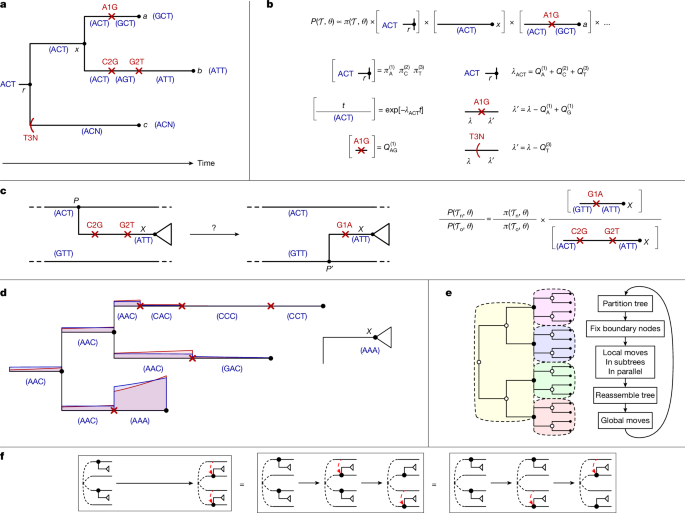
Delphy represents trees internally as a collection of explicitly timed nodes and a reference sequence. Each non-root node points to an earlier parent, and each inner node to two later children. Every instant in the tree has an associated sequence, encoded as successive differences from a reference sequence consisting of L states, each in For more tech updates, stay tuned to our blog.. The root node stores mutations (a,ℓ,b) recording a difference at site ℓ between the reference state a and the root sequence state b; we refer to these mutations as being above the root node. Every other node is annotated with a sequence of mutations from its parent to itself. Each mutation (a,ℓ,b,t) records a change in state at time t from a to b. Thus, the sequence at point x on the tree is obtained starting with the reference sequence, applying the mutations above the root node to obtain the root sequence, then successively applying in order all mutations on the unique path from the root node to x.

Nodes are also annotated with missations, tuples (a, ℓ) recording that for all tips downstream of this node, but not its parent, the state of site ℓ is unknown (missing, ‘N’ in the input); at the parent, the state is a. The tree topology, mutational history and tip sequences jointly completely determine all missations. Missations are encoded using two complementary structures: an ordered sequence of disjoint, non-consecutive half-open intervals [ℓ_start, ℓ_end); and a map of sites ℓ to states a whenever the reference state is not a. This representation reflects that missing data typically appears in a few long gaps, and that the site-to-state map is sparse, as the state at site ℓ is typically the root state when root-to-tip times are small compared with mutation rates (assuming a reference sequence matching a representative root sequence).

To support uncertain tip dates, each tip has a minimum and maximum time, which coincide when there is no uncertainty.

EMATs have evident consistency requirements for node times, mutation times and identities and missation states (Supplementary Information).

Posterior distribution

Delphy samples trees \(Keep following us for the latest insights.\) and associated model parameters θ using MCMC according to the following (unnormalized) posterior distribution:

The factors are as follows:

• \({\pi }_{\theta }(\theta )\) is the prior distribution for the model parameters θ.

• \({\pi }_{{\rm{a}}{\rm{n}}{\rm{c}}}({\mathcal{T}}\,|\theta )\) is an ancestry prior for the tree’s topology given the model parameters θ.

• \(G({\mathcal{T}}\,|\theta )\) is a genetic prior for the particular mutational history decorating the EMAT \({\mathcal{T}}\).

• \(L({\mathcal{T}}\,)\) is the likelihood of the data given the EMAT \({\mathcal{T}}\); as Delphy currently restricts tip sequences to be either definite (A,C,G,T) or completely missing (N), this likelihood is simply 1 if the EMAT is consistent (see above) or 0 otherwise.

The first two priors are described below. The genetic prior is the probability that a random root sequence evolved with the evolution model parametrized by \(\theta \) produces the mutational history in EMAT \({\mathcal{T}}\). Explicitly,

where:

• \({Q}_{{ab}}^{({\ell })}\) is the rate at which state a at site ℓ transitions to state b, as parametrized by the evolutionary model parameters in θ.

• \({Q}_{a}^{({\ell })}=-{Q}_{{aa}}^{({\ell })}\) is the rate at which state a at site ℓ transitions to any other state.

• \({s}_{x}^{({\ell })}\) is the state of site ℓ at point x on \({\mathcal{T}}\).

• \(\xi (x)\) is the set of sites for which at least one tip below point x on \({\mathcal{T}}\) is informative (that is, its state is not missing).

• \(\lambda (x)=\sum _{{\ell }\in \xi (x)}{Q}_{{s}_{x}^{({\ell })}}^{({\ell })}\) is the sequence-dependent genome-wide mutation rate at point x on \({\mathcal{T}}\) (see the N-pruning discussion below).

• \({\int }_{x\in {\mathcal{T}}}f(x){\rm{d}}x\) is an integral of a function \(f(x)\) defined at every point on the tree, defined as the sum of time integrals along each branch of \({\mathcal{T}}\).

• \({\pi }_{a}^{({\ell })}\) is the probability that the root sequence has state a at site ℓ.

• \(r\) is the root node of the tree.

• \({\mathcal{M}}\) is the set of all mutations across the tree.

The Supplementary Information further discusses the motivation for these choices, considerations for efficient calculations and its equivalence to the standard tree likelihood based on Felsenstein pruning.

Parameter and ancestry priors

Delphy’s priors, \({\pi }_{\theta }(\theta )\) and \({\pi }_{{\rm{a}}{\rm{n}}{\rm{c}}}({\mathcal{T}}\,|\theta )\), are currently as follows:

• Tip times are, a priori, uniformly distributed between their minimum and maximum times.

• The transition rate matrices have the form \({Q}_{{ab}}^{({\ell })}=\mu {\nu }^{({\ell })}{q}_{{ab}}\), where μ is an overall per-site mutation rate, the quantities {ν^(ℓ)} are site-relative rates, and \({q}_{{ab}}\) are the normalized transition rate matrix elements of an HKY evolution model with transition-transversion rate κ and stationary state frequencies \({\pi }_{a}\). This form implies a strict molecular clock.

• By default, the mutation rate μ has an improper uniform prior; a more general gamma prior can also be applied.

• The site-relative rates {ν^(ℓ)} are either fixed to 1 (no site-rate heterogeneity), or have a priori \({\nu }^{({\ell })} \sim \mathrm{Gamma}(\alpha ,\alpha )\), with \(\alpha \sim \mathrm{Expo}(1)\) a priori, where ~ means ‘distributed as’.

• The HKY parameters are chosen such that, a priori, \(\{{\pi }_{a}\} \sim \mathrm{Dir}(\mathrm{1,1,1,1})\) and \(\log (\kappa ) \sim N(1,{1.25}^{2})\).

• The ancestry prior is one of:

1. (1)

   A standard coalescent prior with an exponentially growing population curve \(N(t)={n}_{0}{{\rm{e}}}^{g(t-{t}_{0})}\), where t₀ is the time of the latest tip. By default, the final effective population size n₀ has an improper 1/x prior, while the growth rate g has a Laplace prior with mean 0.001 per year and scale 30.701135 per year. More general priors for n₀ and g are also available (Supplementary Information).

2. (2)

   A standard Skygrid flexible population prior⁵¹, where the log of the population curve is specified parametrically at a fixed number of equally spaced times, and at intermediate times is either piecewise constant but discontinuous (staircase, standard) or piecewise linear and continuous (log-linear, particular to Delphy). A priori, the parametrized log-populations follow a random walk with a diffusion constant that allows the population to change by somewhere between halving and doubling in 1 month. We deviate from the original Skygrid by defaulting to fixing instead of inferring this diffusion constant (equivalently, the precision parameter τ), which we find to be both more generally stable and to better encode our intuition of what constitutes reasonable population fluctuations. We also add a penalty for the population curve to assume unrealistically low values (coalescence times below 1 day), which further stabilizes Skygrid for general use. An optional Inverse-Gamma prior can also be applied to the mean population level. Full details are provided in the Supplementary Information.

These choices are suitable for most viral outbreaks, and are currently fixed in Delphy, but their details are not essential. We expect to evolve Delphy to make prior specification more flexible in the future. Most of the above details are the same as the defaults provided by BEAUTi2, and coincide with those used previously²². The priors are discussed further in the Supplementary Information.

MCMC moves

Delphy samples trees and model parameters from the above posterior distribution using MCMC. We distinguish between local moves that affect only a few nodes, and global moves that affect the whole tree.

The following global moves are used (details are provided in the ‘Global moves’ section of the Supplementary Information): Gibbs sampling of mutation rate; delta-exchange moves for stationary frequencies π_a and scale moves for κ; scale moves for α after integrating out {ν^(ℓ)}, followed by Gibbs sampling of {ν^(ℓ)}; population parameter moves (exponential model: scale moves on n₀ and random walk on g; Skygrid: Gibbs move on overall population size, Hamiltonian Monte Carlo move on log-population sizes and optional Gibbs sampling of τ). The relative simplicity of global moves in the explicit-mutation representation, including the marginalization of {ν^(ℓ)} for making moves for α, was first highlighted in ref. ³⁷.

The following local moves are used (details are provided in the ‘Local moves’ section of the Supplementary Information): inner node displacement, branch reform, SPR. For SPR, the regrafting point P′ is proposed using an annealed, approximate mdSPR, scanning points up to 1 mutation away from P in 99% of cases, the whole tree (partition) in 1% of cases. The mutational history on the P′–X branch is a Jukes–Cantor history compatible with end-point sequences, implemented to scale with the number of sequence differences, not the genome size. The interaction of SPR moves with N-pruning is described in full in the Supplementary Information.

Missing data: N-pruning and missations

Missing data substantially complicates using an explicit-mutation representation. Imputing missing data and inferring full mutational histories can be costly in practice (Supplementary Information 5). N-pruning performs Felsenstein pruning only below missations, where the tree likelihood is manifestly 1: the state a below a missation (a,ℓ) evolves to something downstream. This limited Felsenstein pruning preserves the properties of the posterior functional form that Delphy exploits: locality and factorizability; on net, it merely restricts \({\ell }\in \xi (x)\) in the above formulas.

Despite the substantial bookkeeping complications (Supplementary Information 6), one can efficiently update missations on trees as subtrees are pruned and regrafted and mutational histories are changed. Missations enter the proposal and acceptance probabilities of all MCMC moves.

Parallelizable coalescent

Delphy augments the usual Kingman coalescent ancestry prior to allow for parallelization (full details are provided in Supplementary Information 9). In particular, terms involving k(t), the number of active lineages at time t, which a priori require a global view of the tree not available within a single partition, are replaced by terms involving k_p(t), the number of active lineages in partition p only, and an auxiliary Gaussian coupling field with carefully chosen distribution whose net effect is to recover the Kingman coalescent. For local moves, the Gaussian field is kept fixed, so different k_p(t)’s can evolve independently. For global moves, when k(t) is known but static, the coupling field can be Gibbs sampled conditioned on k(t).

To implement this scheme numerically, the Kingman coalescent integral must be discretized at a user-tuneable resolution, below which k(t) and N(t) are approximated as constant. Delphy aims for a discretization with around 400 cells, occasionally changing resolution if the tree height spans too many or too few cells. This default value is often suitable, but can lead to artifacts when there are too many active branches (Extended Data Fig. 4). Note also that there is a subtle interaction between the tree partitioning and correct sampling that must be mitigated in concrete implementations (Supplementary Information 9.1).

While the above scheme is correct and permits parallelization, we expect and encourage better parallelization schemes to be developed.

Lineage and mutation prevalence curves

Delphy’s interface shows prevalence curves u(t) for lineages and mutations, equal to the probability that a random member of the population at time t is descended from the subtree below a lineage’s founding inner node, or one below a specific mutation. The coalescent model yields a simple differential equation for u(t), which Delphy solves numerically (full details are provided in Supplementary Information 12). At densely sampled times, where there are many active lineages k(t), then u(t) reduces to the fraction of active lineages with a certain property. More generally, u(t) is an exponentially moving average of that fraction, with decay rate k(t)/N(t).

Prevalence curves are calculated for each posterior tree, and the mean and 95% HPD range of each such family of curves is displayed to the user.

Automatic detection of burn-in cut-off

Delphy implements a simple heuristic for suggesting an MCMC burn-in cut-off. For a given observable, it calculates the mean and s.d. over the second half of the run, finds the latest time that the observable’s fluctuations exceed 5 s.d., then finds the earliest subsequent time that fluctuations fall within 2 s.d. This time is the suggested cut-off for that observable; Delphy takes the maximum suggested cut-off across the log-posterior, mutation rate and total evolutionary time traces. Unless a user overrides this suggestion, the cut-off is continuously updated; typically, it stabilizes once the run is well into production.

This heuristic identifies a point near the end of the initial burn-in, then advances to the earliest subsequent ‘normal’ part of the trace. Empirically, this procedure makes similar choices as a human would. Importantly for Delphy’s accessibility goal, the cut-off suggestion is made automatically: experience with early users showed that requiring manual cut-off selection led to either needless friction or no cut-off at all, biasing the results.

Delphy input formats

Delphy reads multiple-sequence alignments (MSAs) in FASTA or MAPLE³¹ format. From each description line, a full sequence ID is extracted after the initial ‘>’ up to the end of the line. The full ID consists of fields separated by vertical bars (‘|’): the first field serves as a short ID for the interface and metadata annotation, the last field is a date specification, and other fields are ignored. A date specification can be an exact date (‘2025-01-24’), a month (‘2025-01’), a year (‘2025’) or a date range (‘2025-01-20/2025-01-24’).

Metadata should be a comma-separated value (.csv) or tab-separated value (.tsv) file with a header row. One column should be called “id” or “accession” (case insensitive), with values matching short sequence IDs from the MSA. The remaining columns may have any names and values. Values may be quoted with double-quotes (“), and missing values may be indicated by an empty entry or the values ‘-’, ‘noknown’ or ‘none’ (case insensitive).

Sample MSA and metadata files can be downloaded for the demos on Delphy’s landing page.

APOBEC3-aware evolution model for mpox

Inspired by previous studies^3,4, Delphy includes a specialized evolution model suitable for mpox sequences, which can be activated in the web interface under “Advanced Options”. In brief, each site is classified as having or lacking APOBEC3 context: a site with state C or T has APOBEC3 context when preceded by a T, whereas a site with state G or A has APOBEC3 context when followed by an A. We then use a Jukes–Cantor model with rate μ, modified in sites with APOBEC3 context so C-to-T and G-to-A mutations occur at a rate μ + μ*. This setup retains the essence of the models of refs. ^3,4 but differs minimally in its details. Full details are provided in the Supplementary Information.

Benchmarks

All benchmarks are in the GitHub and Zenodo data repositories (Data availability). Each benchmark is organized as a series of numbered scripts. Unless noted, the scripts are self-contained and download external data as needed. The repos also include intermediate and final results files, as well as many of the plots here and in the Supplementary Information (large files are only at Zenodo; and, for GISAID data subject to its data use agreement, we include download instructions but not the actual data). We intend this repository to be executable documentation of every benchmark detail: while all scripts ran correctly at publication, we do not intend to modify them to ensure they continue to run indefinitely.

We used Delphy v.1.1.4 (build 2044, commit a50e378), MAFFT v.7.505 (10 April 2022), BEAST2 v.2.7.7, BEAST X v.10.5.0, Sapling v.0.1.1 (build 2, commit a0b9da1), BEAGLE commit 6480ad3 (Monday, 15 September 2025), IQ-TREE v.2.3.6 and TreeTime v.0.11.4. The sars-cov-2-gisaid-week-by-week and sims benchmarks used Delphy v.1.0 (build 2036, commit 06a7ee4), which lacks a Skygrid population model but is otherwise not materially different. Unless noted, all calculations were run on AWS c7a.2xlarge instances (eight vCPUs), not the web interface (which is 2–3× slower due to WebAssembly). All Delphy runs were performed twice independently, with convergence checked visually using Tracer⁵⁶.

MCCs were calculated using clade fingerprinting (Supplementary Information), implemented in the ‘delphy-mcc’ utility program that is part of Delphy. We verified these match TreeAnnotator2’s output¹⁵, which hit severe runtime and memory limits on larger benchmarks; by contrast, delphy-mcc processed our 100,000-sequence simulations in minutes. Delphy-mcc applies a 30% burn-in and behaves as if the option ‘–heights ca’ had been given to TreeAnnotator2, so inner node times are the mean tMRCA of the downstream tips over all posterior trees, not just those trees where these tips form a monophyletic clade⁵⁷ (matching the MCC in figure 3a of ref. ²²).

Sampling speed was assessed by dividing ESSs by the wallclock time. For numerical observables, we used LogAnalyser2 (ref. ¹⁵) with 30% burn-in (verified to suffice by visual inspection of traces, and higher than necessary to avoid subtleties relating to incomplete filtering of burn-in). For tree topology, we implemented the frechetCorrelationESS measure described previously⁵⁸, which quantifies the rate at which pairwise Robinson–Foulds distances between trees tend to their long-term expected value with increasing separation in the run (using clade fingerprinting, we can calculate frechetCorrelationESS for even the large H5N1 benchmark in seconds; Supplementary Information 11.2). In all cases, ESS values were in the hundreds to thousands; exact values are in the benchmark repository.

Clade correlation graphs between any two runs (Fig. 2e) were computed using a custom program (compare_clades in the data repo), inspired by the analogous CladeSetComparator tool⁴⁷ in BEAST 2 but using clade fingerprints (Supplementary Information). In brief, we first identify all clades appearing in any posterior sample of either run, and filter out any clade with posterior support below 1% in both runs. We then plot for each clade either the posterior support (Support) or the mean clade tMRCA (tMRCAs) in one run versus the other. Error bars show standard errors for posterior support and mean tMRCAs. Dot areas are proportional to the clade size.

SARS-CoV-2 data from ref. ²² (sars-cov-2-lemieux)

We obtained accession IDs for the 772 samples in figure 3a of ref. ²² from the authors (sample_ids.csv), then downloaded the 757 publicly available sequences in GenBank. These were aligned to reference NC_045512.2 (dated to December 2019) using mafft⁵⁹ (–auto–keeplength), then masked the initial 267 and final 230 sites as in ref. ²².

Delphy was run twice for 2 billion steps (trace every 100,000 steps, posterior trees every 1,000,000). BEAST X and BEAST 2 were run using Delphy’s ‘equivalent’ XML output without changes for 200 million steps (a rough heuristic: 10 Delphy steps achieve the work of 1 BEAST step). Separate runs were prepared with and without site-rate heterogeneity enabled. Two additional BEAST X runs used K = 2 and K = 8 discrete gamma categories for site-rate heterogeneity.

An unrooted ML tree was built with IQ-Tree 2 (-m HKY+FO or -m HKY+FO+G4), then rooted and dated with TreeTime, which also estimates population growth rates (–coalescent skyline –n-skyline 2 –stochastic-resolve).

MCCs were plotted using baltic library, with inner node metadata inferred through parsimony (ties resolved arbitrarily).

Zika data from ref. ² (zika-metsky-2017)

We extracted the sequences from ref. ² from the BEAST XML file in its supplementary data (SupplementaryData/BEAST input and output/Phylogenetic analyses and model selection/SRD06-strict-exponential.xml). These were aligned to reference KX197192.1, with the initial 107 and final 428 sites trimmed. Runs and analysis otherwise follow the SARS-CoV-2 benchmark above.

Ebola data from ref. ¹ (ebola-gire-2014)

We extracted the sequences from ref. ¹ from the BEAST XML file in supplementary file 3 (beast/2014_GN.SL_SRD.HKY_strict_ctmc.exp.xml). In this XML file, the raw sequences are partitioned into genic and intergenic regions, scrambling the mapping to reference KJ660346; we manually deduced the inverse mapping to reconstitute an MSA against this reference. Runs and analysis otherwise follow the SARS-CoV-2 benchmark above.

Ebola data from ref. ²¹ (ebola-dudas-2017)

We extracted aligned sequences and metadata from ref. ²¹ from the companion GitHub repository (Data/Makona_1610_genomes_2016-06-23.fasta and Data/Makona_1610_metadata_2016-06-23.csv at https://github.com/ebov/space-time.git, commit 9db59a4). Runs and analysis follow the SARS-CoV-2 benchmark above, except with longer runs (Delphy: 10 billion steps; BEAST X: 1 million) and a Skygrid population model having 24 month-long intervals over the 2 years ending at the latest tip (24 October 2015), with a log-space random walk prior having a 6-month halving/doubling time (precision τ = 12.3 when effective population sizes are in years).

Mpox data from ref. ³ (mpox-otoole-2023)

We extracted the sequences from ref. ³ from a BEAST XML file in its companion GitHub repository (data/apobec3_2partition.epoch.xml at https://github.com/hmpxv/apobec3, commit c0b4c9b). We removed one non-public GISAID sequence (EPI_ISL_13983888), and two pre-spillover sequences from before 2017 (KJ642617 from 1971 and KJ642615 from 1978), leaving 41 sequences forming the ‘hMPXV-1’ ingroup in figure 3c of ref. ³. The XML partitions sites into APOBEC3-context and remaining sites; since every site is marked ‘N’ in at least one partition, the original aligned sequences are trivially reconstituted.

Delphy was run twice for 200 million steps using –v0-mpox-hack, with trace output every 20,000 steps and posterior trees every 200,000 steps. MCCs and ESSs were calculated as described above.

Mpox data from ref. ⁴ (mpox-parker-2025)

We extracted the sequences from ref. ⁴ from a BEAST XML file in its companion GitHub repository (BEAST/Mpox_2epoch_combinedDTA.xml.zip at https://github.com/andersen-lab/Mpox_West_Africa, commit 2b481da). We removed three non-public GISAID sequences (EPIISL-13953610, EPIISL-13983888 and EPIISL-15008577), and all pre-spillover/pre-2017 sequences, leaving 177 sequences forming the hMPXV-1 clade in ref. ⁴. As above, the XML partitions sites into APOBEC3-context and remaining, so original sequences are trivially reconstituted.

Delphy was run twice for 1 billion steps using –v0-mpox-hack, with trace output every 100,000 steps and posterior trees every 1,000,000 steps. MCCs and ESSs were calculated as described above.

For BEAST comparisons, we modified the original BEAST X XML (BEAST/Mpox_2epoch_combinedDTA.xml.zip) to match Delphy’s sequences and removed phylogeography, spillover detection and pre/post-spillover partitioning. We shortened the chain to 50 million steps, sufficient for convergence (posterior ESS = 374). The script to modify this input file and the resulting XML are in our data repository (mpox-parker-2025-beast.xml).

SARS-CoV-2 data from GISAID submitted/collected by each CDC week (sars-cov-2-gisaid-week-by-week)

We downloaded all SARS-CoV-2 sequences from GISAID collected on or before 31 March 2020 with metadata, filtering out non-human hosts, sequences shorter than 20,000 bases, or with uncertain dates. Each Fig. 5 CDC Epiweek panel includes sequences with the submission date in or before that week (filtered to those submitted in 1 December to 28 March 2020, which is the end of CDC Epiweek 2020-13, and collected from 1 December 2019). For Supplementary Fig. 7, we used collection date instead of submission date (and filtered sequences to those submitted in 1 December 2019 to 31 December 2024, and collected from 1 December 2019). Matching sequences were aligned to NC_045512.2 using mafft, then masked at the initial 268 and final 230 sites (as described previously²²). No further masking was applied.

Quick initial diagnostic runs revealed clear outlier sequences (for example, inducing a tMRCA to early 2019, lying in an isolated long branch with tens to hundreds of mutations, collection dates far preceding first reported cases in a particular region). After several rounds of iterative refinement by outlier removal, no trees contained obvious outliers. We verified that most offending sequences had been identified as outliers near the beginning of the pandemic, marked as under investigation in GISAID, or appeared in NextStrain or sarscov2phylo exclusion lists. See Supplementary Tables 1 and 2 for the 94 excluded sequences.

Delphy was run on AWS c7a.4xlarge instances (16 vCPUs) for each Epiweek as in the SARS-CoV-2 benchmark, with the following differences: 5 million steps per tip, 10,000 trace and 200 tree samples and at most 1 thread per 100 tips (maximum 32 threads).

Simulated trees for scaling assessment (sims)

We prepared two groups of four SARS-CoV-2-like simulated datasets with N = 100, 1,000, 10,000 and 100,000 tips. The first group used an exponentially growing population curve, \(N(t)={n}_{0}\,{e}^{g(t-{t}_{0})}\) with n₀ = 6 years, g = 10 per year and t₀ = 31 July 2024. The second used a constant population N(t) = n₀ = 2 years. Sample times were drawn from [1 January 2024, 31 July 2024] proportional to N(t), mimicking a uniform sampling of members of the historical viral population, then linked through a standard coalescent simulation. A random 30,000-site root sequence was sampled with π = [0.30, 0.18, 0.20, 0.32] and evolved along the ancestry using the Gillespie algorithm under a site-homogeneous HKY model (mutation rate, 1 × 10⁻³ per site per year, κ = 5). Trees were recorded in Newick format, summaries in JSON, and dated tip sequences as FASTA (N ≤ 1,000) and MAPLE files. To perform these simulations efficiently, we wrote a tool called sapling (Code availability, Data availability and Supplementary Information 15.2).

Delphy was run twice on a 96-vCPU c7a.24xlarge AWS instance with 5 million steps per tip, 10,000 log and 200 tree samples and at most 1 thread per 20 tips (maximum 192 threads). The n = 100,000 run also used around 10,000 cells for discretizing the coalescent prior instead of the default about 400 (comparisons at 625–5,000 cells are shown in Extended Data Fig. 4).

H5N1 in cattle dataset (h5n1-andersen-2025)

We cloned the Andersen laboratories avian-influenza repository from GitHub (https://github.com/andersen-lab/avian-influenza) at commit e756a15 (3 October 2025). From 11,541 unique SRRs, we filtered to the 4,080 non-retracted SRRs with a cattle host and B3.13 genotype. For each of H5N1’s 8 segments, we aligned to reference A/cattle/Texas/24-008749-003/2024 (SRR28752635), as found in ‘avian-influenza/reference’, using mafft, then concatenated the segments longest-to-shortest into a single sequence per sample (assuming no appreciable reassortment, which appears valid as of October 2025).

For dating, we identified the 3,339 sequences with GenBank accessions providing day-resolved dates (SRR metadata dates typically only indicate year). We prepared these as input to Delphy; runs with the larger set that includes those with uncertain dates exhibited severe convergence problems and were excluded. For geographical analysis, we used GenBank’s ‘geo_loc_name’, which resolves to a US state in 3,194 of 3,383 accessions.

Delphy was run twice for 20 billion steps (trace every 2 million steps, trees every 20 million). We applied a Skygrid model with 22 month-long intervals ending at the latest tip (5 August 2025), with a log-space random walk prior with 3 month halving/doubling time (precision τ = 6.15 when effective population sizes are in years). Coalescent prior discretization was increased to 1,000 cells to reduce discretization error.

Reporting summary

Further information on research design is available in the Nature Portfolio Reporting Summary linked to this article.