Plant material

Plants of R. tenuis and R. austrobrasiliensis were collected from natural populations in Brazil under appropriate permits and cultivated under controlled greenhouse conditions. Nine geographically distinct accessions of R. tenuis were used for genome sequencing and cytological analyses. Individual flowers and pollen were staged for meiotic analyses. All experimental material was propagated clonally from field-collected individuals to ensure genetic identity across assays.

Sequencing

High-molecular-mass DNA was extracted from young leaf tissue using a modified cetyltrimethylammonium bromide protocol. PacBio HiFi libraries were prepared and sequenced on the Sequel IIe platform. Illumina short-read sequencing was used for genome polishing and transcriptome profiling. Hi-C libraries were constructed using Arima Hi-C kits and sequenced on the Illumina NovaSeq 6000 platform. RNA was extracted from young inflorescences for expression analyses.

DNA isolation

High-molecular-mass DNA from R. tenuis and R. austrobrasiliensis was isolated from 1.5 g of material using the NucleoBond HMW DNA kit (Macherey Nagel). Quality was assessed using a FEMTO-pulse device (Agilent), and the quantity was measured using the Quantus Fluorometer (Promega).

PacBio

HiFi libraries were prepared according to the ‘Preparing whole genome and metagenome libraries using SMRTbell prep kit 3.0’ manual, with an initial DNA fragmentation by Megaruptor-3 (Diagenode) and final size-selection by BluePippin (Sage Science). Size distribution was again controlled by FEMTO-pulse (Agilent). Size-selected libraries were then sequenced on a Revio device using the Revio polymerase kit and Revio chemistry for 30 h (Pacific Biosciences).

Arima Hi-C

Plant tissues were cross-linked with 1% formaldehyde for 30 min at room temperature, and the reaction was quenched with 125 mM glycine for 10 min. Subsequently, the tissues were ground using a TissueLyser at a frequency of 30 Hz for 3 min. Nucleus extraction was performed using the CelLytic PN Plant Nuclei Isolation/Extraction Kit (Sigma-Aldrich) according to the manufacturer’s protocol. Hi-C libraries were prepared using the Arima High Coverage Hi-C Kit (Arima Genomics, A410110) according to the manufacturer’s instructions, and were then sequenced (paired-end, 2 × 150 bp) on the NextSeq 2000 instrument (Illumina).

Methyl-seq analysis

To investigate the methylome space in R. tenuis (REC accession), the relatively non-destructive NEBNext Enzymatic Methyl-seq Kit was used to prepare an Illumina-compatible library, and paired-end sequencing (2 × 150 bp) was performed on the NextSeq 2000 (Illumina) instrument. For each library, 10 Gb of reads was generated.

RNA-seq analysis

Total RNA was isolated from flower buds (REC accession). Poly(A) RNA was enriched from 1 μg total RNA using the NEBNext Poly(A) mRNA Magnetic Isolation Module. RNA-seq libraries were prepared as described in the NEBNext Ultra II Directional RNA Library Prep Kit for Illumina (New England Biolabs). A total of 11 cycles was applied to enrich the library concentration. Sequencing was performed at BGI Genomics using the BGISEQ-500 system on the DNBseq platform in paired-end mode with a read length of 2 × 150 bp.

Illumina libraries (TPase and DNA FS)

Genomic DNA from 49 and 59 controlled self-crossed R. tenuis REC and PECP35-7 accessions, respectively, were deep-sequenced on the Illumina HiSeq 3000 system or, alternatively, using DNBseq short-read sequencing (BGI Genomics) in 150 bp paired-end mode.

k-Mer-based haplotype divergence estimation

Heterozygosity levels of R. breviuscula, R. austrobrasiliensis and all R. tenuis accessions were estimated by GenomeScope2.0 (ref. ⁵⁴). k-Mer counting was performed using FASTK (v.1.1; https://github.com/thegenemyers/FASTK) with PacBio HiFi reads, which were used for genome assembly, as the input. The k-mer size was 31 (Fastk -k31). The resulting binary output (.hist) from FASTK was then converted to a text histogram file by Histex (part of FASTK): Histex -G hifi_31mer.hist > hifi_31mer.histo. The histogram was then analysed with GenomeScope2 using k = 31 and ploidy=2, except for R. austrobrasiliensis, for which ploidy = 6.

To avoid ambiguity, we interpret the GenomeScope estimate as a reference-free measure of haplotype divergence rather than as strict SNP heterozygosity. GenomeScope infers this value from the k-mer frequency spectrum by modelling the relative contribution of haplotype-specific and shared k-mers. Thus, the estimate captures sequence differences that generate haplotype-specific k-mers, including SNPs, indels and unique haplotype-specific regions, but it may treat repetitive divergent sequence differently from unique sequence. We therefore use this value as a complementary measure of genome-wide haplotype divergence, particularly useful in R. tenuis, where highly divergent or structurally variable regions may be excluded from alignment-based estimates.

Genome assemblies

HiFi reads were assembled using Hifiasm (v.0.25.0) with the default settings, combining both PacBio HiFi reads and Hi-C reads to generate haplotype-resolved contigs. The assembly quality was assessed using BUSCO (v.5.2.2)⁵⁵ and QUAST (v.5.3.0)⁵⁶. Duplicated haplotypes were retained for downstream analysis.

Scaffolding

Chromosome-scale scaffolding was performed using the Juicer and 3D-DNA pipelines^57,58. Contigs from each haplotype generated from HiFiasm were taken as Hi-C alignment targets. Hi-C contact maps were visualized using Juicebox Assembly Tools to manually curate misjoins and validate the final pseudomolecules. Haplotypes were scaffolded independently and phased using k-mer-based alignment strategies.

k-Mer completeness and assembly artefact evaluation

To evaluate whether haplotype size discrepancies reflected true biological variation rather than assembly artefacts or missing sequence, we performed k-mer completeness and copy-number spectrum analyses using Merqury (v.1.3). For each accession, 19-mers were derived from raw PacBio HiFi reads using Meryl (canu v.2.1). We evaluated k-mer multiplicity distributions across individual haplotype assemblies (h1 and h2) and the combined diploid assembly. Assembly completeness and structural integrity were confirmed by inspecting the presence of unrepresented read k-mers (read-only k-mers) relative to expected heterozygous (1×) and homozygous (2×) coverage peaks. A 2× multiplicity peak in the isolated h1 spectrum representing shared homozygous k-mers was omitted from h2. The absence of read-only k-mer peaks at heterozygous and homozygous coverage positions in the diploid spectrum confirms high assembly completeness across both haplotypes, demonstrating that observed haplotype size differences represent genuine structural variation rather than differential assembly collapse or gapped repetitive regions.

Gene-based synteny analysis

Genes used for synteny analysis were annotated by a deep-learning-based tool Helixer (v.0.3.4)^59,60 with the land plant mode. Gene synteny was analysed for R. breviuscula haplotype 1, R. austrobrasiliensis haplotype 1, and all haplotypes of nine R. tenuis accessions using GENESPACE (v.1.3.1)⁶¹ running in R (v.4.2.0) along with the dependent tools OrthorFinder (v.2.5.5)⁶² and MCScanX (v.1.0.0)⁶³. The R script for running GENESPACE (run_genespace.R) can be found in our project GitHub page (https://github.com/Raina-M/Rhynchospora_tenuis_project).

DNA sequence-based synteny analysis

Collinearity of all R. tenuis haplotypes was analysed by SyRI (v.1.5.3)⁶⁴. The alignment between haplotypes was conducted using minimap2 (v.2.28)^65,66 with the following parameter settings: -ax asm5 –eqx. The plot was generated using plotsr (v.0.5.3) with a minimal 50 kb syntenic block size. NOR regions labelled on the haplotypes were searched by BLAST (v.2.12.0) with the Arabidopsis rDNA sequences as the template.

Pangenome analysis

Pangenomes were generated using minigraph (v.0.17) with phased chromosome-scale assemblies from nine accessions. Variants were extracted using vg toolkit v.1.40.0. Structural variants and sequence divergence were quantified across homologous haplotypes. Repeat annotation was performed with DANTE (v.0.2.10) and DANTE_LTR (v.0.4.0.5)⁶⁷ and EDTA (v.2.0)⁶⁸ using the plant TE library. Pairwise divergence and TE composition were visualized using custom R scripts.

PanKmer analysis and haplotype clustering

To evaluate haplotype conservation and relationships across all 18 R. tenuis haplotypes, pangenome k-mer profiling was conducted using PanKmer (v.0.20.4). An index of canonical 31-mers was constructed from the assembled fasta files for all accessions using ‘pankmer index’. Pairwise sequence overlaps were subsequently quantified by generating an adjacency matrix with ‘pankmer adj-matrix’. To visualize haplotype relationships, hierarchical clustering was performed on the matrix through ‘pankmer clustermap’ using the Jaccard similarity index as the distance metric, yielding an adjacency clustermap in which the colour intensity reflects the average nucleotide similarity across haplotypes (Extended Data Fig. 4a).

Pseudogene analysis

RNA sequences were mapped to diploid R. tenuis REC and R. breviuscula by STAR (v.2.7.11b). RNA data for R. breviuscula was from our previous publication¹⁷. The gene annotations from Helixer with at least one RNA coverage were taken as functional genes. All functional genes, repeats and TEs were hard-masked. We used miniprot (v.0.18) to map the functional gene sequences to the hard-masked genome then parse the output with our custom script. Only alignments matching a ≥40% sequence identity and ≥50% query coverage threshold were considered. Alignments displaying at least one inactivating open reading frame (ORF) disruption (frameshifts or premature stops) were classified using structural criteria: (1) processed pseudogenes required an intronless, compact footprint (≤2 CDS blocks and a genomic span ≤1.20× the expected mRNA length); (2) non-processed pseudogenes were identified by a retained multi-exon structure or non-compact genomic span. Scripts are available in our GitHub repository (folder: search_pseudogenes; https://github.com/Raina-M/Rhynchospora_tenuis_project).

ChIP–seq

Chromatin immunoprecipitation (ChIP) was performed as described previously⁶⁹ with minor modifications. Young leaves and flower buds were collected from greenhouse-grown plants and immediately frozen in liquid nitrogen before storage at −80 °C. Tissue samples were cross-linked with 4% formaldehyde under a vacuum on ice for 1 h, and the reaction was quenched by adding 1 M glycine. Nuclei were isolated using NIB buffer (50 mM HEPES pH 7.4, 5 mM MgCl₂, 25 mM NaCl, 5% sucrose, 30% glycerol, 0.25% Triton X-100, 0.1 % β-mercaptoethanol and 0.1% protease inhibitor), and chromatin was extracted in TE-SDS buffer. Chromatin was sheared by sonication for 30 s on/30 s off cycles for a total of 25 cycles. For immunoprecipitation, the sonicated chromatin was incubated overnight at 4 °C with 2 ng of the following antibodies: anti-CENH3⁷⁰, anti-H3K4me3 (Abcam, ab8580), anti-H3K9me2 (Abcam, ab1220) and anti-H3K27me3 (Merck, 07-449). A control without antibodies was performed simultaneously. The antibody–chromatin complexes were captured using rProtein A Sepharose Fast Flow (Sigma-Aldrich, GE17-1279-01) or Protein G Sepharose 4 Fast Flow (Sigma-Aldrich, GE17-0618-01). Bound chromatin was eluted, and de-cross-linked by treatment with proteinase K. DNA was purified by ethanol/sodium acetate precipitation and resuspended in nuclease-free water. The purified DNA was sent for library preparation and sequencing.

Sequencing reads were aligned to the reference genome using Bowtie2⁷¹ using the –very-sensitive-local option. ChIP and control alignments were compared using bamCompare⁷² with the parameters –binSize 50 –normalizeUsing RPKM –operation log2. The resulting log₂ ratio tracks were visualized using pyGenomeTracks⁷³. Metaplots were generated using computeMatrix⁷² (scale-regions mode) with the parameters –regionBodyLength 20000 –beforeRegionStartLength 10000 –afterRegionStartLength 10000 –binSize 50, and plotted using plotHeatmap. The mean of each column of the matrix over Tyba arrays was extracted, which is the actual value plotted on the metaplots. As all epigenetic signals (CENH3, H3K4me3, H3K9me2, CG, CHG and CHH methylation) are not normally distributed (Shapiro–Wilk normality test P < 0.05), we performed spearman correlation analysis between every signal in R. pubera, R. breviuscula and R. tenuis to test whether these signals present the same pattern across different species.

Probe design and oligo-FISH

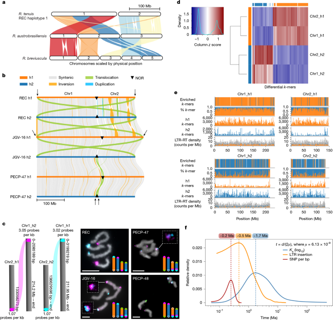
After phased genome assembly and synteny analysis, a haplotype-specific translocation in R. tenuis reference plant was identified at the chromosome ends. To validate these data, we designed oligo probes specific to each translocated region and hybridized in the reference plant, in different accessions, plus R. austrobrasiliensis. Probes were designed for the following regions to each chromosome/haplotype: for chromosome 1 (Chr1_h1, 0–3100219 bp; Chr1_h2, 0–2085189 bp) at a density of 3 probes per kb (Fig. 1c), and for chromosome 2 (Chr2_h1, 133059273 bp to end; Chr2_h2, 136628596 bp to end) at a density of 1 probe per kb. After designing and setting the regions corresponding to each haplotype, these data were submitted to Daicel Arbor Biosciences for synthesis and labelling of the probes. Probes for haplotype 1 were labelled with Atto633 (far red), while probes for haplotype two were labelled with Alexa Fluor 488 (green). For the slide preparation, young roots (mitosis) and flower buds (meiosis and microgametogenesis), from plants maintained in pots at greenhouse facilities of Max-Planck Institute for plant Breeding Research, were collected and fixed in Carnoy solution (methanol:acetic acid, 3:1, v/v) for 2–24 h at room temperature and then immediately used or kept at −20 °C until the moment of use. After fixation, the material was digested in enzymatic solution containing 2% cellulase Onozuka (Serva), 2% pectolyase Y-23 (Duchefa Biochemie), 2% cyto-helicase (Sigma-Aldrich) and 10% pectinase (Sigma-Aldrich) in citrate-phosphate buffer (pH 4.5), washed in water and macerated in 60% acetic acid, post-fixed with ice-cold fresh Carnoy solution and air dried. For removal of cytoplasm, the slides were washed in 60% acetic acid for at least 30 min, then air dried. For the pollen tube germination experiment, 30 mature flower buds were collected into 3 ml of sterile distilled H₂O and vortexed to release pollen grains. From the bottom of the tube, 300 µl of the pollen suspension was collected and added to 3 ml of liquid medium for trinucleate pollen as described previously⁷⁴. Pollen grains were incubated at 28 °C for 24 h. After incubation, the medium containing germinating pollen grains was transferred into a conical tube and centrifuged at 5,000 rpm for 3 min. After removing the supernatant, pollen nuclei were suspended in 60% acetoacetate, transferred onto a slide, post-fixed and air-dried. For oligo-FISH, the procedures were similar to the ones described previously⁷⁵; in brief, the hybridization mix was composed of 50% formamide (Sigma-Aldrich), 2× SSC (saline sodium citrate) solution (pH 7.0), 10% dextran sulfate, 350 ng of probe labelled in Alexa Fluor 488 and 200 ng of the probe labelled in Atto633 (a total of 15 µl per slide). After denaturation and hybridization, the slides were passed through stringency washes in 2× and 0.1× SSC at 42 °C, which corresponds to a final stringency of about 76%. The slides were counterstained with 2 µg ml⁻¹ DAPI in Vectashield H-100 antifade mounting medium (Vector Laboratories) and photographed on the Zeiss Microscope coupled with a Zeiss Axio Imager 2 camera system and software ZEN Blue (v.3.1). Images were treated in brightness and contrast using Adobe Photoshop software.

Immunocytochemistry

Immunocytochemistry was performed as described previously¹⁸, with some variations. In brief, young flowers of R. tenuis and R. austrobrasiliensis were sampled and fixed in ice-cold 4% (w/v) paraformaldehyde (PFA) in PBS solution (pH 7.5, 1.3 M NaCl, 70 mM Na₂HPO₄, 30 mM NaH₂PO₄) and 0.1% (v/v) Triton X-100 for 30 min in a vacuum. Flowers were dissected to select anthers of the appropriate size to obtain meiocytes in prophase I. Anthers were opened from the tip in a drop of PBS with 0.1% (v/v) Triton X-100 and squeezed to release the meiocytes from the locules. The suspension of meiocytes was stirred to separate individual nuclei and remove excess debris. A coverslip was pressed onto the suspension to squash the meiocytes and later removed with liquid nitrogen. Slides were mounted with Vectashield containing 0.2 µg ml⁻¹ DAPI and checked for prophase I stages of interest. Selected slides were incubated with blocking buffer (3% (w/v) BSA in PBS + 0.1% (v/v) Triton X-100) for 1 h at 37 °C to block and permeabilize the cells. The following antibodies were used: anti-AtASY1 raised in rabbit (PAK006)²⁴, anti-AtMLH1 raised in rabbit (PAK017)²⁷ and anti-AtZYP1-cter raised in chicken (PAK053). Another anti-RpZYP1 was raised in rat against the peptide KLTAERLVKDQASVKNDLEC (gene ID: RP1G00482580, RP4G01479980, RP2G00810370, RP5G01738420) and affinity-purified (Lifeprotein). The anti-RpREC8 was a combination of two antibodies raised in rabbit against the peptides CEEPYGEIQISKGPNM and CYNPDDSVERMRDDPG (gene ID: RP1G00316120/RP2G00915110, RP4G01319620, RP5G01638170) and affinity-purified (Eurogentec)¹⁸. The anti-RpHEI10 was a combination of four antibodies raised in rabbit and rat against the peptides CNRPNQSRARTNMFQL, CPVRQRNNKSMVSGGP, CIDIMDSRDMLRQGKREREEIW and CDTDSAVNMGPPSGDTSNRR (gene ID: RP3G01271190, RP3G01008630, RP1G00269340, RP2G00699130) and affinity-purified (Eurogentec and Lifeprotein)¹⁸. Primary antibodies were diluted in the blocking buffer to a final volume ratio of 1:200. Slides were incubated with primary antibodies overnight at 4 °C. The next day, the slides were washed three times for 5 min each with PBS + 0.1% (v/v) Triton X-100. The samples were incubated with secondary antibodies for 2 h at room temperature or 1 h at 37 °C. Secondary antibodies were conjugated with STAR ORANGE (Abberior, STORANGE-1007) or Alexa Fluor 488 (Thermo Fisher Scientific, goat anti-rabbit IgG (H+L), Superclonal Recombinant Secondary Antibody, A27034) diluted 1:250 in blocking buffer. The slides were washed again three times for 5 min with PBS + 0.1% (v/v) Triton X-100 and allowed to dry. The samples were then prepared with 10 µl of mounting solution (Vectashield + 0.2 µg ml⁻¹ DAPI). Specimens were covered with a coverslip and sealed with nail polish for storage. Images were taken with a Zeiss Axio Imager Z2 with Apotome system for optical sectioning. Images were deconvolved and processed with ZEN Blue (v.3.1) software and Adobe Photoshop (v.27.0.0).

Image processing and analysis

To measure the degree of fragmentation of the SC of R. tenuis compared with R. austrobrasiliensis, deconvolved nuclei at zygotene for both species were selected. The ZYP1 signal was isolated and converted to 8-bit in FIJI. The signal threshold was adjusted based on the maximum entropy and the signal was skeletonized. The skeleton number representing the fragment number and branch lengths representing SC elongation were extrapolated. For each cell, the number of skeletons was divided by the total length of the SC. We named the resulting value the SC fragmentation coefficient, representing the degree of fragmentation of the SC signal per unit of SC length (Supplementary Fig. 9a). To measure the ability of recombination proteins to form foci, deconvolved nuclei at diakinesis were selected. ZEN Blue software (v.3.1) was used to analyse the histograms of MLH1 and HEI10 signals. The skewedness of the distribution of pixel intensities was used as a measurement of tendency to form foci, as high-intensity foci skew the distribution of pixels towards higher intensities (Supplementary Fig. 9b,c). To measure the ability of HEI10 and MLH1 signals to colocalize, deconvolved nuclei at diakinesis were analysed using the colocalization tool in ZEN. Quadrants were adjusted based on Costes test for statistical significance, and the Pearson’s colocalization coefficient was extrapolated (Supplementary Fig. 9d). R scripts used for the plots are available at Zenodo (https://doi.org/10.5281/zenodo.20847664).

Meiotic gene analysis

Meiotic genes with a role specifically in meiotic recombination were selected from the literature based on plants and other eukaryotes. Sequences were selected from Arabidopsis or closer relatives in the case of poorly conserved genes (for example, rice, maize, barley). Protein sequences were used as a query for TBLASTN with our in-house genomes, annotations and expression datasets. The number of hits on the same query sequence was used as a starting measure of copy number. The results were then manually curated for validation (Supplementary Fig. 15). Expression evidence for meiotic genes was based on the analysis of the inflorescence transcriptome obtained by RNA-seq data.

To further evaluate SHOC1 transcriptional activity, flower buds of R. tenuis (REC and PECP-47 accessions), R. breviuscula and R. austrobrasiliensis were used for total RNA isolation using the Sigma-Aldrich Spectrum Plant Total RNA-Kit (STRN50-1KT) together with the On-Column DNase I Digestion Set (DNASE70-1SET). Isolated RNA (1 μg) was used for cDNA synthesis using the Thermo Scientific RevertAid First Strand cDNA-Synthesis-Kit (K1622). The obtained cDNA was used for qPCR analysis using the NEB Luna Universal qPCR Master Mix (M3003S) on the BIO-RAD CFX96 Real-Time PCR Detection System. List of oligos is provided in Supplementary Table 5.

Epigenomic profiles at the SHOC1 locus were examined using newly generated chromatin and DNA methylation datasets. For R. tenuis, tracks corresponding to histone modifications (H3K4me3, H3K9me2 and H3K27me3), RNA-seq coverage and DNA methylation levels (CG, CHG and CHH contexts) were visualized for both haplotypes using pyGenomeTrack⁷³ views centred on the annotated SHOC1 gene. DNA methylation profiles were derived from whole-genome enzymatic methylation sequencing datasets, and RNA-seq from flower buds data were used to assess transcriptional activity at the locus. For comparison, epigenomic data for the orthologous SHOC1 locus in R. breviuscula were obtained from published datasets¹⁸. All tracks were visualized and compared using the same genomic window to assess transcriptional activity and methylation patterns across species.

Pollen nucleus isolation and sequencing

The protocol was adapted from a previous study¹⁸. For collecting the pollen, mature flowers of R. tenuis were collected into 5 ml tubes containing woody pollen buffer (scWPB: 200 mM Tris-HCl, 4 mM MgCl₂, 2 mM EDTA, 86 mM NaCl, 10 mM Na₂S₂O₅, 250 mM sucrose, 0.5 mM spermine, 0.5 mM spermidine; 1% PVP-10), and vortexed for 30 s at maximum speed. The obtained solution was filtered through a 50 µm CellTrics cell strainer into a 5 ml tube. The samples were centrifuged at 5,000g for 5 min, the supernatant was removed and the pollen pellet was frozen in liquid nitrogen. Pollen viability was assessed by Alexander staining (Morphisto, 13441-00250). Pollen samples were stored at −70 °C until further use.

For extracting the pollen nuclei, frozen pollen samples were thawed on ice for 5 min and resuspended in scWPB. The solution was filtered through a 5 µm CellTrics cell strainer, retaining the pollen. Pollen grains inside the cell strainer were crushed with a plastic rod. Pollen nuclei were filtered from the macerated pollen by adding scWPB with some additives to preserve RNA (scWPC; 5 mM DTT, 1%BSA, 0.2 U µl⁻¹ Protector RNase Inhibitor). Pollen nucleus solution was stained with DAPI (1 µg µl⁻¹) and used for fluorescence-activated cell sorting (FACS) to enrich the nucleus population. A BD FACSAriaIII Fusion Flow Cytometer with a 70 µm nozzle and 483 kPa sheath pressure, operated with BD FACSDiva software (v.8.0.3), was used for this purpose; the sequential gating strategy is shown in Supplementary Fig. 16. Nuclei were dispensed into a 96-well plate containing collection buffer (1× PBS, 1% BSA and 0.2 U µl⁻¹ Protector RNase Inhibitor). The quality and number of nuclei were evaluated with the LUNA-FX7 Automated Cell Counter. Nucleus solutions were used for library preparation using Chromium Next GEM Single Cell ATAC or Chromium Next GEM Single Cell 5′ Kits according to the manufacturer’s instructions. Libraries were sequenced at BGI Genomics according to the Chromium 10x Kit recommendations.

Single-cell analysis

Single-cell RNA data were analysed with a similar pipeline reported in the previous study in R. breviuscula¹⁸. The genotyping markers were defined by haplotype-specific polymorphisms by remapping the PacBio HiFi reads that were used for genome assembly to the assembled haplotype 1 genome then calling SNPs. Remapping was implemented by minimap2 (v.2.28) with argument options: -ax map-hifi. SNPs were called by bcftools (v.1.9): (1) bcftools mpileup -Oz –min-MQ 1; then (2) bcftools call -Avm -Oz. The output VCF file was converted by ‘SHOREmap convert’ (v.3.6) to extract three key pieces information on alternative alleles: mapping quality, read coverage and AF. Only the alternate alleles with mapping quality over 100, read coverage and AF close to the main peaks were used as markers for genotyping. All snRNA-seq data were first analysed using cellranger (v.9.0.1), and snATAC data were analysed using cellranger-atac (v.2.1.0). The output alignment file (.bam) from cellranger was then demultiplexed to single-cell alignment files based on barcodes. We next called variants in each cell and compared them with genotyping markers, based on which we can determine the genotype along the chromosomes. Crossover was then called when a genotyping switch occurred. A full description of the pipeline and parameters is provided at GitHub (https://github.com/Raina-M/detectCO_by_scRNAseq).

Statistical analysis of segregation distortion

Differences between observed and expected gamete genotype frequencies were assessed using χ² goodness-of-fit tests, considering only the three detectable NOR-bearing genotype classes. The expected frequencies were calculated assuming equal transmission among these classes under random segregation in inverted achiasmatic meiosis. The NOR-null class was excluded because it was not observed among viable pollen grains or sperm cells. Statistical analyses were performed in R.

Subgenome-aware phasing of R. tenuis haplotypes

We used SubPhaser²² (default parameters) to phase and partition the haplotypes of R. tenuis by assigning chromosomes to subgenomes based on differential repetitive k-mers. These were assumed to have expanded during the period of independent evolution after the loss of recombination. A subgenome is considered to be well phased when it displays distinct patterns of both differential k-mers and homoeologous chromosomes, confirming the presence of subgenome-specific features.

Estimating divergence times between haplotypes

Divergence times between haplotypes were estimated using the method outlined previously⁷⁶. In brief, all SNPs, derived from SyRI (v.1.5.3)⁶⁴ analysis explained above, between two haplotypes were used to estimate divergence times according to the formula g = d/2μ, where g is the number of generations, μ is the assumed mutation rate of 6.13 × 10⁻⁹ (ref. ²³), and d is the number of SNPs per bp (d = total number of SNPs between two haplotypes/chromosome size). We assumed a generation time of one per year.

LTR insertion times were calculated by Subphaser as follows: LTR-RTs were de novo detected using LTRharvest (v.1.6.1)⁷⁷ and LTRfinder (v.1.07)⁷⁸. To reduce false positives, TEsorter (v.1.3.0)⁷⁹ was used to reconstruct the classification of LTR-RTs and further refine this classification. The subgenome-specific k-mer sequences were mapped to the LTR-RT sequences using a substring match procedure to identify the subgenome-specific LTR-RTs using Fisher’s exact test. Two LTRs of each subgenome-specific LTR-RT were retrieved and the nucleotide divergence was estimated using the Jukes–Cantor 1969 model. The insertion time (T) was calculated using the equation T = K/2r, where r = 6.13 × 10⁻⁹ substitutions per year, and K represents the divergence of the LTRs from the LTR-RT.

The K_s between two haplotypes was computed based on the CDS sequences annotated by Helixer by CoGe (https://ghibli.bti.cornell.edu/coge/). Genomes and gene annotations were uploaded to CoGe, and the option to calculate K_s was selected during the SynMap run. All K_s values of coding sequences that overlapped with TE annotation were removed by ‘bedtools subtract -A’.

Phylogenetic tree construction

The phylogenetic tree was built based on single-copy orthologues (SCOs) among R. breviuscula, R. austrobrasiliensis and all haplotypes of R. tenuis. SCOs were extracted from the output of OrthoFinder (v.2.5.5) in GENESPACE (v.1.3.1). All SCO groups were aligned by MAFFT (v.7.475)⁸⁰ with the parameter ‘–auto –maxiterate 10’. All alignments were concatenated with a custom Python script available at our project GitHub page (phylogeny_based_on_SCOs/concatenate_aln.py). The tree was constructed based on the catenated alignments with RAxML-NG (v.1.2.2)⁸¹, then visualized in FigTree (v.1.4.4) (https://github.com/rambaut/figtree/).

F₁ genotyping and analysis

F₁ individuals were obtained from selfed heterozygous mother plants. Genomic DNA from seedlings was extracted and sequenced on the Illumina NovaSeq platform. The F₁ genotyping method was the same as described previously¹⁸. Whole-genome sequencing reads of each F₁ offspring were mapped to the haplotype 1 assembly using bowtie2 (v.2.5.1) paired-end mode and the default parameters, and SNP genotypes were called afterwards using bcftools (v.1.9), whereby we first performed ‘bcftools mpileup’ then then ‘bcftools call -Am’. The resulting SNPs of each individual plant were compared with the defined genotyping markers (see the ‘Single-cell analysis’ section) to determine the genotypes of all genomic regions along each chromosome. Genotyping results were cross-validated by TIGER and RTIGER (v.2.1.0). RTIGER was implemented under R (v.4.2.0) and Julia (v.1.0.5).

The crossed F₁ individuals were sequenced by Illumina short reads, which were then aligned to the mother genome assembly with haplotype 1 and 2 catenated by bowtie2 (v.2.5.1) in paired read mode with the option ‘–local –no-mixed –no-discordant’. The alignment file was sorted by samtools sort (v.1.24). SNP calling was performed using the bcftools (v.1.9) mpile up with the option –min-MQ 1 and then bcftools call -Avm. The output VCF file was converted by SHOREmap convert (v.3.6) into a text format file, where the AF of alternative alleles/SNPs can be read. Only alternate alleles with AF > 0.95 and coverage > 3 were extracted as valid SNPs, that is, the alleles called in the cross reads are truly different from the mother alleles. These alleles were compared with the SNPs output by SyRI (v.1.5.3), which mapped father diploid genome assembly to mother diploid genome assembly. The overlapped SNPs indicate they are contributed by father (Fig. 4b).

Gene conversion detection in selfed F₁ plants

To detect gene conversions in selfed individuals, we calculated the alternative (hap2) AF based on the SNP markers used for genotyping. Markers with a combined read depth below 5× were excluded. We then applied binomial test at each marker site with total depth as sample size n and number of reads supporting hap2 as number of successful trials k. The null hypothesis is that the hap2 allele count at a given marker site follows a binomial distribution. To control the false-discovery rate genome wide, every testable marker was assigned a raw P value and the Benjamini–Hochberg procedure was applied globally across all SNP markers on all chromosomes simultaneously. We next merged neighbouring significant SNPs into tracts, and only tracts of 5 bp–5 kb were considered to be potential gene conversions. However, if total depth drops at the same positions relative to flanking sites, we took it as a deletion or hemizygosity rather than conversion, because conversion usually preserves depth but changes the allele fraction. The related R script is available on our project GitHub page (detect_gene_conversion.R). Although the pipeline excluded as many biases and false positives as possible, manual inspection of reported gene conversions with alignments in IGV was performed.

Embryo and endosperm analysis

For extracting the nuclei from embryo and endosperm, frozen seeds were macerated with a plastic rod and resuspended in seed nucleus isolation buffer (100 mM Tris, 5.2 mM MgCl₂, 85.55 mM NaCl, 0.1% Triton X-100, 0.2 U µl⁻¹ Protector RNase Inhibitor, pH 7.5). The obtained solution was filtered through a 20 µm CellTrics cell strainer into a fresh 2 ml tube and stained with DAPI (1 µg µl⁻¹). A BD FACSAriaIII Fusion Flow Cytometer with a 70 µm nozzle, operated with BD FACSDiva software (v.8.0.3), was used for FACS to enrich the 2c (embryo) and 3c (endosperm) nucleus populations; the sequential gating strategy is shown in Supplementary Fig. 16. The separate 2c and 3c nucleus populations were dispensed into a 96-well plate containing collection buffer (1× PBS, 1% BSA, and 0.2 U µl⁻¹ Protector RNase Inhibitor). The quality and number of nuclei were evaluated using the LUNA-FX7 Automated Cell Counter. Nuclei solutions were used for library preparation using Chromium Next GEM Single Cell ATAC according to the manufacturer’s instructions. Libraries were sequenced at BGI Genomics according to the Chromium 10x kit recommendations.

Female gametophyte sectioning and imaging

Developing ovaries and whole inflorescences were fixed as described previously³⁴. Dehydration and infiltration into Araldite 502/Embed 812 resin were performed in an EMS LYNX II automated tissue processor (EMS). After resin polymerization, serial semithin sections (1 µm) were produced from ovules at different stages of development, stained with 1% aqueous Toluidine Blue supplemented with 1% sodium tetraborate and imaged on the Zeiss Axio Imager M2 system. Images were stacked and aligned in FIJI/ImageJ (v.2.18.0) using the StackReg plugin (BIG-EPFL). MorphoGraphX (v.2.0.3) was used for 3D rendering of the aligned images and volumetric visualization of the embryo sac tissue⁸². Three-dimensional segmentation of the embryo sac was performed using ITK watershed (https://www.itk.org) in MorphoGraphX, taking PlantSeg (v.2.1.1)⁸³ predictions from the ‘generic confocal 3DUNET model’ as input images for 3D cell segmentation. Immunodetection of β-1,3-glucan to identify pollen tube cell walls was performed as described previously⁸⁴, with the exception that BSA was omitted from the buffer during all steps. Goat anti-mouse Alexa Fluor 647 (Abcam, ab150119) was used as an alternative secondary antibody at a dilution of 1:200. Imaging was done on the Leica SP8 system using LAS X (v.5.3.3).

For Feulgen staining of siliques, the pericarp was removed from the mature and fertile siliques; for the rest of the siliques, the pericarp was not removed, and the material was fixed in ethanol:acetic acid (3:1) overnight. The samples were washed three times with distilled water for 15 min each wash and then incubated in 5 N HCl for 1 h, followed by another series of three washes with water, as before. The siliques were then incubated in Schiff’s reagent for 3–4 h, after which they were washed three times with cold distilled water (4 °C). Next, the siliques were incubated in ethanol series 10 min each, 10%, 30%, 50%, 70%, 95% and then washed several times with 99.5% ethanol until the ethanol came out colourless. The samples were incubated in a 99.5% ethanol:LR White resin series (3:1 then 2:1), 15 min for each solution. The samples were then incubated for 1 h in ethanol:LR White resin (1:1), followed by an overnight incubation in LR White resin. The seeds were next mounted onto microscope slides in LR White resin and polymerized for 24 h at 60 °C. Feulgen-stained samples were imaged using the Leica Stellaris 8 or Leica SP8 FALCON Dive multiphoton microscope using LAS X (v.5.3.3). Samples were excited at either 800 nm or 1,060 nm, and emission was collected from 580 to 700 nm.

Reporting summary

Further information on research design is available in the Nature Portfolio Reporting Summary linked to this article.