Animals

Wild-type C57BL/6J female and male mice (2–6 months old; Jackson Laboratory) were used as experimental animals. Mice were housed under a reversed 12 h–12 h light–dark cycle (lights off at 07:00 and on at 19:00) in a temperature- and humidity-controlled environment (18–23 °C, 40–60% humidity), with ad libitum access to food and water. Training began when mice were approximately 2–3 months of age. All pairs were age-matched at the start of training. During training and experiments, mice were water restricted but maintained at 80–90% of their initial body weights. Experiments were conducted during the dark cycle, and each training session lasted for about 1 h, during which mice received 0.5–1.5 ml of water from the task. Animals received supplemental water as necessary to maintain their body weights. All procedures complied with the National Institutes of Health Guide for the Care and Use of Laboratory Animals and were approved by the Icahn School of Medicine at Mount Sinai Institutional Animal Care and Use Committee.

Behavioural apparatus

The training arena was an 18 inch × 18 inch white-acrylic square chamber. Four reward zones were positioned at the centre of each arena wall, each with two adjacent water delivery ports. Reward ports were 3D-printed using white and transparent resins, each incorporating an infrared beam for nose-poke detection and a white LED to indicate its availability. Water was delivered through a stainless-steel tube within each port, controlled by a solenoid valve (Lee, LHDB0533418H). An initiation detector, fitted with an infrared LED and a reflective sensor, was positioned at the centre of the arena to detect trial initiation when approached by mice. Analogue signals from all ports were digitized through the Arduino Nano and acquired through a DAQ system (National Instruments, USB-6001). Behavioural control was implemented in LabVIEW (National Instruments, 2014) to manage trial timing, LED signalling, water delivery and data logging. Mouse behaviour was recorded at 30 fps using an overhead camera (Teledyne FLIR, BFS-U3-16S2M-CS).

Video tracking

We used the machine-learning-based tools SLEAP (v1.3.3)⁵⁵ and Ensemble Kalman Smoother (EKS) (v0.0.0)⁵⁶ to annotate the nose, neck and torso positions of both mice in each video frame, enabling precise tracking of their movement and posture. To identify individual mice, we shaved a small patch of back fur on one mouse in each pair. Each mouse was annotated with three key points: nose (tip of the nose), neck (centre of the neck) and torso (centre of mass), which were connected to form a skeleton. Approximately 4,200 video frames from 10 mouse pairs were manually annotated for training a SLEAP model, which was then used to automatically estimate the key points of other pairs. To optimize tracking accuracy, we additionally applied EKS—a post-processing method that refines pose estimation outputs by smoothing several model predictions, resulting in more robust tracking. Custom MATLAB scripts (MathWorks, 2024b) were used to align the behaviour data from LabVIEW with the video frames based on the LED onset and offset.

Behavioural definitions

Mouse position was defined using its neck position, which was also used to calculate speed and acceleration. The reward zone was defined as a semicircle with a 10 cm radius centred at the midpoint between each pair of reward ports (Extended Data Fig. 1h). Arrival was defined as the first frame in which a mouse’s neck position entered a reward zone. Reaction time was defined as the time from trial onset to arrival at the chosen reward zone.

Cooperative foraging task training

Before training, mice were water restricted to 1 ml per day for at least 3 days and habituated to the experimenter and the behavioural set-up. Mice underwent one training session per day, progressing through four main stages.

Stage 1: light-guided water retrieval

Mice were trained to associate illuminated ports with water rewards within a single reward zone, separated from the rest of the arena by an acrylic barrier. On each trial, the left or right port in that reward zone was randomly illuminated; poking the illuminated port triggered water delivery and turned off the light. Mice advanced to stage 2 after 3 days of training.

Stage 2: learning to initiate trials

Mice were given access to the entire arena, including all four reward zones and the central initiation point. Trials began when a mouse was detected by the sensor at the initiation point, triggering illumination of both ports in a single active reward zone. Mice were required to poke an illuminated port within 15 s to receive a water reward; poking an inactive port terminated the trial and was followed by a timeout (6–10 s). Mice that reached 80% correct progressed to stage 3.

Stage 3: cooperative foraging shaping

Two same-sex cage mates (not necessarily siblings) that completed stage 2 were introduced to the arena together. Either mouse could initiate a trial, illuminating both reward ports within a single reward zone. Mice were required to each poke an illuminated port in the same zone within 15 s to receive a reward. The two mice may arrive at different times, and one can wait for the other, but the reward is delivered only when both mice nose-poke simultaneously. Poking an inactive port by either mouse terminated the trial and triggered a timeout (6–10 s). Mice that reached 80% correct advanced to stage 4a.

Stage 4a: cooperative foraging training

On each trial, either mouse could initiate by crossing a central initiation point, which standardized the position of that mouse at trial onset. The partner’s position was unconstrained and naturally variable, enabling assessment of how one animal’s spatial state influences the other’s decision-making. After trial initiation, two of the four reward zones were randomly illuminated as active zones. To receive a water reward, both mice were required to choose the same reward zone, each nose poking into one of its two ports (the match rule). As in stage 3, the two mice may arrive at different times, and one can wait for the other, but reward is delivered only when both mice nose-poke simultaneously. We refer to this joint action by two agents towards a shared goal as cooperation.

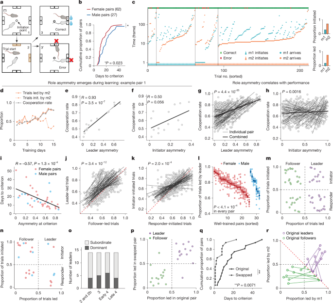
Trials were terminated without reward if the two mice chose ports from different active zones (mismatch error) or if either mouse poked any port from an inactive zone (unrewarded error). All error trials were followed by a timeout (6–10 s) added to the inter-trial interval (ITI, 3–8 s) before the next trial. Omitted trials are defined as failure to respond within 15 s in early stage 4a or within 8 s in late stage 4a. The correct rate is defined as the number of correct trials divided by all trials excluding omitted trials. Criterion performance is defined as 80% correct across three consecutive sessions, and pairs are excluded if they do not reach criterion after 50 days of training.

Social role assignment

Once a pair reached the training criterion (≥80% correct rate for three consecutive sessions), we assigned each mouse as either a leader or follower, and independently as an initiator or responder. To determine leadership, we computed the proportion of trials led by one mouse in a session and compared it to chance (0.5) using a two-tailed binomial test (α = 0.01). If the proportion was significantly biased, the mouse that led more trials was designated the leader; otherwise, no leader was assigned. The same procedure was applied to assign initiators and responders. Leader asymmetry was defined as the absolute difference between the proportion of trials led by each mouse; initiator asymmetry was defined analogously for trial initiation. Importantly, these classifications reflect role biases over sessions rather than fixed identities: leaders may follow and responders may initiate on a small subset of trials. Unrewarded errors and omitted trials were excluded from analysis, as leader and follower roles could not be assigned in these trials, and both occurred infrequently (0.5% and 1.2%, respectively, during the well-trained stage; Extended Data Fig. 1b,c). Accordingly, we evaluated mouse performance in these analyses using correct and mismatch trials only and defined a cooperation rate as the proportion of correct trials relative to the sum of correct and mismatch trials.

Manual annotation of behavioural motifs

Trial start and end times were extracted from the behavioural recordings to segment the continuous video into individual trials. A 30-frame pre-trial buffer was appended to each segment to provide temporal context. Segmented trials were concatenated into a single video (5–15 min in duration) for manual annotation. Videos were then annotated frame by frame by trained observers using Avidemux (v.2.8.1). For each identified behavioural motif, the start and end frame numbers were recorded. We then mapped these indices to corresponding frames in the original video and generated Gantt charts for visual inspection. Motifs were quality-checked and excluded if they exceeded a predefined duration threshold or occurred during the ITI.

The following four social behavioural motifs were defined and manually annotated. All behavioural motifs reflect pairwise interactions, but the track, sharp turn and join motifs were attributed to the actor mouse that performed the action. The synchronized travel motif was not assigned to either mouse, as it involved joint, symmetric behaviour.

Synchronized travel

The two mice move in parallel, maintaining similar linear and angular velocities and a consistent close distance throughout the trajectory. They arrive at the same reward zone in a coordinated, synchronized manner.

Track

One mouse, while initially approaching an active reward zone, slows down and turns its head to monitor the movement of its more distant partner. After detecting the partner’s approach, it adjusts its timing to allow both animals to arrive at the reward ports nearly simultaneously.

Sharp turn

Each mouse initially moves towards a different active reward zone. During the approach, one mouse abruptly changes its trajectory by more than 90°, redirecting its movement towards the reward zone selected by the partner.

Join

One mouse initiates movement towards an active zone independently. The partner mouse, initially stationary or undecided, subsequently aligns its trajectory with the first mouse after observing its movement. Both animals then travel together towards the same reward zone.

Partner swapping

Groups of four same-sex cage mates were randomly assigned to two dyads for cooperative foraging training. Once both pairs reached the training criterion and the social roles were assigned, we swapped partners either by pairing the leader from one dyad and the follower from the other (Fig. 1p,q and Extended Data Fig. 4a–d), or by pairing both leaders or both followers (Fig. 1r and Extended Data Fig. 4e–k). If both mice in a new pair were shaved, we marked one with black dye (Stoelting, 50450) for tracking with SLEAP. We then resumed training with the new pairs until they again reached the training criterion.

Solo foraging control (stage 2b)

Solo foraging was typically performed after stage 2 to assess the reward zone preferences of individual mice in the absence of a partner. After initiation, two reward zones were randomly illuminated, and the mouse received water by poking any port from the active zones. Poking an inactive port ended the trial without a reward and was followed by a timeout.

Cooperative foraging with rule reversal (stage 4d)

In stage 4d, task contingency was reversed: mice were rewarded for choosing different active zones (the mismatch rule). Choosing the same reward zone terminated the trial without reward. All other task parameters remained unchanged. A subset of mouse pairs well-trained in stage 4a was retrained in stage 4d.

Non-social stimulus tracking task

For the non-social-stimulus-tracking task (Fig. 3n), the behavioural arena was identical to that used for cooperative foraging, except that the opaque floor was replaced with a transparent base. A projector positioned beneath the arena projected a visual stimulus onto the floor through a mirror and filters. Before training, mice were water restricted and habituated to the experimenter and apparatus as described above. Training consisted of four stages.

Stage 1: single-zone reward acquisition

Mice were trained to obtain water rewards from a single active reward zone. On each trial, a black elliptical visual stimulus (3 × 6 cm) appeared at the centre of the arena and remained stationary for 0.5 s before moving towards the reward zone along a straight trajectory with small jitter orthogonal to the direction of motion. After reaching the reward zone, the stimulus remained at the port for 5 s while rotating. A nose poke at one of the corresponding reward ports within this response window triggered water delivery. Failure to respond was recorded as an error and followed by a 6 s timeout. The ITI was 3 s. Mice typically advanced to the next stage after approximately 3 days of training.

Stage 2: initiation training

Mice were trained to voluntarily initiate trials by crossing the central initiation point. After initiation, the visual stimulus appeared at the centre for 0.5 s before moving towards the single active reward zone as in stage 1. A correct trial required a nose poke at one of the corresponding reward ports within a 5 s response window. Incorrect responses were followed by a 6 s timeout. Mice that reached 80% correct progressed to stage 3.

Stage 3: two-choice tracking

Two adjacent reward zones were made available. After trial initiation, the stimulus appeared at the centre for 0.5 s and then moved to one of the two active reward zones, selected randomly. Mice were required to track the moving stimulus and poke one of the corresponding reward ports within a 5 s response window to receive a reward. Incorrect trials were followed by a 6 s timeout. Mice typically advanced after approximately 5–6 days of training.

Stage 4: trajectory-based stimulus tracking

This stage approximated the spatial and temporal structure of the cooperative foraging task. All four reward zones were made available. Instead of moving along a straight path, the stimulus replayed trajectories drawn from a library of 20 well-trained cooperative foraging sessions. The library included both leader and follower trajectories from trials initiated by the animal, ensuring that each replayed trajectory began at the centre of the arena. On each trial, one trajectory was randomly selected (50% chance from the leader pool and 50% from the follower pool) and replayed from the centre towards the corresponding reward port. The reward was delivered if the mouse poked the same reward zone towards which the stimulus was directed within the response window; otherwise, the trial was terminated and followed by a 6 s timeout. Training continued until performance plateaued, defined as less than 5% variation in the correct rate across three consecutive sessions.

Dominance hierarchy assays

To determine hierarchy, we used three independent and well-established assays: the tube test⁵⁷, warm spot test^22,23 and reward competition test^24,25. These assays probe competitive interactions under different behavioural contexts to provide convergent measures of dominance hierarchy.

Tube test

The tube test was performed in a round-robin design with groups of four cage mates to assess dominance hierarchy. In a subset of animals, tube tests were repeated at multiple training stages (stage 2/2b, stage 3, early stage 4a and well-trained stage 4a) to assess the relationship between leader–follower roles and dominance hierarchy at each stage. In some cases, the tube test was performed within the two-animal pair only, which was sufficient for assessing the relationship between dominance hierarchy and leader/follower role assignment. During the test, mice were placed at opposite ends of a transparent acrylic tube (12 inches long, 1.25 inches in diameter) and encouraged to enter. As only one mouse could pass through the tube at a time, the mouse that forced the other to retreat was designated the dominant individual. In the round-robin design, each four-animal group completed six rounds of pairwise testing, and testing continued daily until a stable hierarchy was observed for four consecutive days.

Warm-spot test

Experiments were conducted in a covered transparent acrylic arena (1 ft × 0.5 ft × 0.5 ft; length × width × height). A black circular plastic platform (2.5 cm in radius) was positioned in one corner of the arena to serve as the warm spot. A small USB heating pad placed beneath the platform provided localized warmth. Cages containing four cage mates were placed on ice together with the test arena for 30 min before testing. Mice were then transferred to the arena and marked individually for identification. Behaviour was recorded for 20 min. The time each mouse spent on the warm spot was quantified using BORIS (v.9.2.3)⁵⁸.

Reward competition test

The reward competition test assessed dominance during direct competition for a limited resource. As mice were well trained on the cooperative foraging task, they readily poked illuminated reward ports without additional training. In this test, a single reward port from the cooperative foraging apparatus was used, and two mice competed for access to the port, with reward availability signalled by LED illumination. Each session consisted of 20 trials with a 3 s ITI. After a 2 day habituation period, the mice were tested in two sessions (one session per day). For cages containing four mice, all pairwise combinations were tested, yielding six matches per day in a randomized order.

Stability criteria

In the tube test, stable social rankings were achieved by design through daily testing for up to 2 weeks, until a consistent hierarchy was established. For the warm-spot test, social rank was considered stable if the ranking, determined by time spent on the warm spot, was identical across two consecutive days. All tested groups reached stability within 2 days, except for one instance in which the relative ranking of two mice reversed. For the reward competition test, stability was defined as one mouse winning at least 60% of all trials summed across the two test sessions²⁵.

Elo score calculation

Dominance hierarchies were quantified using a sequential Elo rating system, originally developed for ranking chess players⁵⁹ and later adapted to estimate dominance hierarchies in animal groups^25,60. The Elo score provides a dynamic, continuous estimate of an individual’s dominance strength within its group and is updated sequentially after each contest. All individuals were initialized with an Elo score of 1,000. After each dyadic interaction between individuals A and B, with current ratings, \(a_a\) and \(_s\), we first calculated the expected probability that A would win:

Ratings were then updated sequentially according to:

where \({R}_{{\rm{A}}}^{{\prime} }\) is the updated score, S_A equals 1 for a win, 0 for a loss and 0.5 for a tie. The parameter K, which determines the sensitivity of rating updates, was set to 20. The rating of individual B, \({R}_{{\rm{B}}}^{{\prime} }\), was updated analogously using \({S}_{{\rm{B}}}=1-{S}_{{\rm{A}}}\) and the corresponding expected probability \({E}_{{\rm{B}}}\).

For the tube test and reward competition test, outcomes were derived from repeated round-robin dyadic contests within each group. The warm spot assay did not involve direct dyadic encounters; instead, the total occupancy time for each individual was ranked within the group, and pairwise outcomes were inferred such that the individual with greater occupancy time was assigned a win in each dyadic comparison. These inferred outcomes were incorporated into the same sequential Elo framework. Final Elo scores were used as continuous measures of relative dominance within each assay and were used to calculate cross-assay correlations in dominance ranking.

Virus

The following viral vectors were purchased from Addgene: AAV8-hSyn-hM4D(Gi)-mCherry (7 × 10¹² viral genomes (vg) per ml; 50475-AAV8), AAV8-CaMKIIα-hM4D(Gi)-mCherry (2 × 10¹² vg per ml; 50477-AAV8), AAV8-hSyn-mCherry (1 × 10¹³ vg per ml; 114472-AAV8), AAV9-syn-jGCaMP8m-WPRE (1 × 10¹³ vg per ml; 162375-AAV9), AAV9-Syn-GCaMP6f-WPRE-SV40 (7 × 10¹² vg per ml; 100837-AAV9) and AAV5-CAG-GFP (7 × 10¹² vg per ml; 37825-AAV5). AAV8-CaMKIIα-KALI1-eYFP (1.8 × 10¹³ vg per ml; GVVC-AAV-292) was obtained from the Stanford University Virus Core.

Stereotaxic surgery

Mice were anaesthetized with a cocktail of ketamine (100 mg per kg) and xylazine (10 mg per kg) and secured in a stereotaxic frame (Kopf Instruments, Model 940). Anaesthesia was maintained with 1–1.5% isoflurane throughout the procedure. Viral injections were performed using a glass capillary connected to a nanoinjector (Drummond Scientific, Nanoject III) at a rate of 1–2 nl s⁻¹. Stereotaxic coordinates were determined according to the Paxinos and Franklin mouse brain atlas. After surgery, mice received either a single dose of the long-acting analgesic buprenorphine (3.25 mg per kg, Ethiqa XR) or carprofen (5 mg per kg) for three consecutive days.

Chemogenetic inactivation of the mPFC was performed using AAV8-hSyn-hM4D(Gi)-mCherry or AAV8-CaMKIIα-hM4D(Gi)-mCherry, with AAV8-hSyn-mCherry as the control. Viral injections were administered at four sites per hemisphere to cover the entire mPFC (bregma coordinates: anteroposterior (AP), +1.98 mm; mediolateral (ML), ±0.45 mm; dorsoventral (DV), −1.85 mm/−1.45 mm, 200 nl per depth; AP, +1.18 mm; ML, ±0.45 mm; DV, −1.10 mm, 300 nl; AP, +0.50 mm; ML, ±0.45 mm; DV, −0.80 mm, 300 nl; AP, −0.20 mm; ML, ±0.45 mm; DV, −0.80 mm, 300 nl). For chemogenetic inactivation of the OFC, 300 nl of AAV8-hSyn-hM4D(Gi)-mCherry was injected bilaterally at AP, +2.46 mm; ML, ±1.00 mm; DV, −1.75 mm.

For optogenetic inactivation of the mPFC, AAV8-CaMKIIα-KALI1-eYFP was used, with AAV5-CAG-GFP as the control. Viral injections were performed at two sites per hemisphere (300 nl per site): AP, +1.98 mm; ML, ±0.45 mm; DV, −1.85 mm/−1.45 mm; and AP, +1.18 mm; ML, ±0.45 mm; DV, −1.10 mm. After injections, bilateral optical fibres (Amuza, TeleLCD-Y-2.0-500-0.9) were implanted at AP, +1.98 mm; ML, ±0.45 mm; DV, −0.80 mm. Optical fibres were secured with black dental acrylic (Lang Dental Manufacturing, Ortho-Jet) to firmly attach the fibre and block external light.

To implant a GRIN (gradient index) lens for miniscope recording, we performed a craniotomy over the mPFC at AP, +1.98 mm; ML, +0.45 mm with a 1-mm-radius window. Brain tissue above the mPFC was aspirated with a 27-gauge blunt or bent needle while continuously irrigating with cortex buffer to preserve tissue integrity. The resulting cavity was shaped to be as close to cylindrical as possible. We then injected 600 nl of AAV9-Syn-jGCaMP8m-WPRE or AAV9-Syn-GCaMP6f-WPRE-SV40 virus unilaterally at AP, +1.98 mm; ML, +0.45 mm; DV, −1.70 mm. After injection, a 1-mm-diameter, 4-mm-length GRIN lens (Inscopix) was positioned at the injection site and implanted 1.45 mm below the brain surface. The lens was secured with cyanoacrylate adhesive (Loctite) and further protected with a layer of low-toxicity silicone adhesive (World Precision Instruments, Kwik-Sil). Finally, dental acrylic was applied to stabilize the implant and cover the remaining exposed skull.

After 2–3 weeks of viral expression, mice were reanaesthetized and placed back into the stereotaxic frame. The overlying dental cement was carefully drilled off to expose the implanted GRIN lens. A Miniscope⁶¹ pre-mounted on a fixed baseplate was positioned above the lens, and the field of view was monitored in real time. The Miniscope was gradually lowered until the imaging field was visible. Once we observed the optimal field of view, the baseplate was secured with cyanoacrylate and dental cement. To minimize interference from external light, an outer layer of black dental cement was applied. A protective cap was then attached with screws, and mice were allowed to recover with postoperative analgesia. Viral expression and implant placement were verified histologically in all animals, and only animals with correct targeting were included in the analyses. Calcium imaging as well as inactivation during cooperative foraging were performed primarily in female pairs, because animals were single-housed after surgery to protect implants and incisions during recovery, and adult males could not be reliably re-paired. The non-social-stimulus-tracking task, which tests individual mice and does not require re-pairing included both sexes.

Chemogenetics

For chemogenetic manipulation, we injected the viral vectors into untrained mice and allowed at least 4 weeks of viral expression while simultaneously training them on the cooperative foraging task. We administered the DREADD agonist clozapine N-oxide (CNO; 5 mg per kg; Tocris, 4936) dissolved in saline through intraperitoneal injection 30 min before the start of the session. We performed the control session on the day before the inactivation session, when we injected mice with an equal volume of saline to control for potential effects of liquid intake and handling. To control for potential non-specific effects of CNO, we administered the same dose to a separate control group expressing mCherry and evaluated their behaviour in the cooperative foraging task.

Wireless optogenetics

We used a wireless optogenetic system (Amuza, Teleopto) for mPFC inactivation. After completing behavioural training, virus injection and fibre implantation surgery, mice were given 2–3 weeks for viral expression and post-surgical recovery. Only mice that reached the training criterion were included in the optogenetic experiments, all conducted within 4 weeks after surgery. Before the stimulation session, animals were fitted with dummy receivers for 3 days during training to acclimatize to the implants and receivers.

For stimulation, a lightweight receiver was connected to the implanted optical fibres. Stimulation signals were generated by a task control system (National Instruments, NI-6001) as transistor–transistor logic (TTL) pulses and transmitted through BNC cables to the optogenetic control unit. The behavioural set-up enabled precise inactivation across different task periods, including throughout the trial and 1 s or 2 s from trial onset. During stimulation sessions, light pulses were delivered on one-third of the trials according to a pseudorandomized schedule. To prevent intensity fluctuations caused by battery discharge, we limited stimulation intensity to one-third of the maximum output of the implanted LED (590 nm, ~0.8 mW per hemisphere). Optogenetic inhibition in both or a single animal was achieved by independently activating the receiver in each mouse.

One-photon calcium imaging

Post-surgical mice with clear imaging fields were selected and trained in the cooperative foraging task. Calcium imaging was performed during well-trained stage 4a of the training protocol. Each day, one mouse underwent calcium imaging while the other was fitted with a dummy scope of equal weight to control for potential impact of the Miniscope attachment. In each recording session, neural activity was recorded from only one animal, either the leader or the follower. Imaging data were acquired using the Miniscope DAQ system and synchronized with behavioural video recordings at 30 fps. A TTL signal generated by the Miniscope DAQ was transmitted through a trigger cable (6-pin GPIO Hirose Connector Cable, FLIR) to the behaviour-recording camera, ensuring frame-by-frame alignment. We used Suite2p⁶² for region-of-interest identification and extraction of calcium transients, and Cascade⁶³ to infer spike rate from the calcium signals. To compute fluorescence changes (ΔF/F), we first subtracted 70% of the local neuropil signal from the fluorescence signal of each cell to obtain the raw trace. To estimate a dynamic baseline, we first smoothed the raw trace using a Gaussian filter with s.d. σ = 6.7 s to reduce high-frequency noise and then applied a two-step filtering process: first, a moving minimum filter with a window size of 500 s was applied to the smoothed trace to track the lower envelope; a moving maximum filter of the same window size was then applied to this result to obtain a conservative estimate of the baseline. ΔF/F was computed by normalizing the raw trace to this dynamic baseline. Analyses of selectivity for choice and leading versus following included 6 animals expressing GCaMP6f and 2 animals expressing GCaMP8m. Spatial selectivity analyses included 6 animals expressing GCaMP6f and 6 animals expressing GCaMP8m. Mice were excluded from calcium imaging analysis if they show incorrect viral targeting, insufficient viral expression, a low-quality field of view or low-quality calcium signals.

Electrophysiological recording

To validate mPFC inactivation, extracellular single-unit recordings were performed acutely in head-fixed animals that expressed the appropriate effector genes. Four animals were used for validating chemogenetic inactivation and three animals for optogenetic inactivation. Recordings used 64-channel silicon probes (Cambridge Neurotech, Acute H3 probe) stereotaxically targeted to the mPFC using Bregma coordinates: AP, 1.78–2.22 mm; ML, 0.45 mm; DV, 1.85–2.30 mm. Before recording, a craniotomy (0.3–0.8 mm in diameter) was performed over the target area, and the recording depth was determined using micromanipulator readings. Data were acquired on the Intan RHD recording system (Intan Technologies) and digitized at 25 kHz. After each recording session, the brain surface was protected with silicone gel (Dow Corning, 3-4680) and Kwik-Sil (World Precision Instruments). Voltage signals were high-pass filtered and automatically sorted using Kilosort3⁶⁴. Spike clusters were then manually curated using the Phy GUI⁶⁵ to merge spikes from the same units and exclude noise and poorly isolated units. Recording sites were visualized by staining the probes with Vybrant DiO (Invitrogen, V22886) or Vybrant DiI (Invitrogen, V22885) and verified histologically after recording.

To validate chemogenetic inactivation, we first recorded a baseline level of activity from animals expressing AAV8-hSyn-hM4D(Gi)-mCherry. We then administered CNO (5 mg per kg, intraperitoneal) while continuing to record, to capture the effect of inactivation. To validate inactivation using KALI-1, we used animals expressing AAV8-CaMKIIα-KALI1-eYFP in the mPFC. An optical fibre (RWD, 0.50 NA, 200 μm diameter) was positioned approximately 0.5 mm above the brain surface, producing an illuminated area with an estimated radius of around 0.3 mm for 590 nm illumination. To prevent collision with the fibre, the recording probe was inserted at a 10-degree angle. The brain surface was illuminated at varying light intensities, with each power level tested 10 times within a recording session (2 s of illumination per light pulse, 30 s between pulses). For validation of the wireless optogenetic device, an optical fibre (Amuza) was implanted at a 10-degree angle, secured 0.5 mm below the brain surface with dental cement. A recording probe was inserted at a 10-degree angle to avoid collision and positioned to record from mPFC neurons beneath the illuminated area.

Unsupervised behavioural classification

We computed LISBET (v0.3.0) embeddings, a self-supervised representation of behaviour that captures body kinematics in a high-dimensional latent space²⁶. Using the pretrained LISBET model, we generated 64-dimensional embeddings for each video frame. As body keypoints were tracked with SLEAP but the pretrained LISBET model was trained on DeepLabCut (DLC) coordinates, we generated pseudo-DLC keypoints by inferring the corresponding DLC body points from the SLEAP-derived coordinates. To prevent embeddings from capturing task-irrelevant information (for example, which of the four reward zones was chosen), we restricted the analysis to correct trials and rotated all trials to a common configuration with the chosen reward zone in the north. Embeddings were computed across all sessions from all mouse pairs using a temporal window of 20 video frames. The target frame included a context of 20 frames into the past.

To quantify the organization of LISBET embeddings with respect to human-defined behavioural motifs, each datapoint was assigned to a cluster corresponding to its manually annotated motif label. We then computed a modified silhouette score for each datapoint \(i\):

where a_i is the mean distance between point i and all points assigned to other clusters, and b_i is the mean distance between point i and all other points within the same cluster. This metric resembles the standard silhouette score, with two modifications that increase sensitivity to structured but non-clustered data: (1) a_i is defined as the mean distance to all points in all other clusters, rather than only to the closest other cluster as in the standard formulation; and (2) the denominator is a_i, rather than max(a_i,b_i). For each mouse pair, silhouette scores were averaged across all frames and sessions to obtain a single summary value.

Spatial decision-making analysis

To examine how a mouse’s decision is influenced by its partner on trials initiated by the mouse of interest, we compared the mouse’s zone choice in the cooperative foraging task to a solo foraging control. For this analysis, all adjacent trial types were rotated to align the active zones to a north-east configuration. Trials longer than 5 s (10.0% of all trials), unrewarded errors (0.5%; Extended Data Fig. 1b) and omitted trials (1.2%; Extended Data Fig. 1c) were excluded.

To visualize the mouse’s choice (Fig. 2f,g and Extended Data Fig. 8a,b), we performed the following logistic regression:

where P_North denotes the probability that the mouse of interest selects the north zone. θ_East and θ_North are the mouse’s absolute head angles relative to the east and north directions, respectively. I_Partner indicates whether the partner is facing a given reward zone (Fig. 2f,g) or whether the partner is located in a given reward zone (Extended Data Fig. 8a,b), depending on the condition. The β terms are fitted coefficients: β₀ captures baseline bias towards the north zone in the solo control (in log-odds units); β₁ and β₂ reflect the animal’s sensitivity to heading information in the solo control (with β₁ > 0, β₂ < 0, in well-trained animals); β₃ quantifies the shift in bias attributable to the partner; and β₄ and β₅ reflect changes in heading sensitivity in the presence of the partner. To visualize the effect of a partner in a given state (for example, facing or located in the east), the regression included only solo trials and cooperative trials matching that state; cooperative trials with the partner in other headings or locations were excluded.

To quantify changes in heading sensitivity and directional bias induced by the presence of the partner (Fig. 2h,i and Extended Data Fig. 8c,d), we first computed a single heading-difference variable:

where larger values indicate greater alignment with the north than the east reward zone. Using the same I_Partner coding, we then fitted the following model separately for leaders and followers within each partner condition:

Similar to equation (4), β₂ quantifies the partner-induced changes in choice bias for the north zone; β₃ estimates the partner-induced changes in sensitivity to the mouse’s own heading. Here I_Partner = 1 for cooperative trials and 0 for solo foraging, with trials selected per partner state as described for equation (4).

To examine the influence of spatial variables on both leader and follower decision-making across all trials in a single framework (Fig. 2p–r and Extended Data Fig. 8o–r), we first calculated the differences in each animal’s heading and distance relative to the two active zones at trial onset, and standardized these values to the range of [0,1] before model fitting:

We then used the following equations to fit the leader and follower’s decision, respectively:

Although the equations are structurally identical, separate β coefficient sets were fit for leaders and followers. We predicted the leader’s and follower’s choice using these logistic fits (Fig. 2q and Extended Data Fig. 8o,q). The GLM was fit to a training set, and the model performance was evaluated on a held-out test set as the proportion of correctly predicted choices. We used 90% of the data for training and 10% for testing, repeated across 100 random splits.

To assess statistical significance, we compared model performance against a shuffled null distribution. For each fold, a shuffled version of the data was created by randomly permuting choice labels, and the model was trained and tested using the same predictor variables. Model accuracy on true versus shuffled data was compared across folds using a bootstrap procedure (10,000 iterations) to estimate the P value for the observed difference in mean accuracy. This procedure was applied separately to predict leader and follower choices, yielding role-specific estimates.

To examine the impact of chemogenetic and optogenetic inactivation on heading sensitivity and choice bias (Fig. 3i,k,m and Extended Data Fig. 11p), we used the following logistic regression to fit the leader or follower’s decision:

where β₆ to β₉ quantify the changes in sensitivity to leader and follower’s heading and distance induced by inactivation. Trials were pooled across sessions and animals to increase the statistical power.

Choice selectivity analysis

To identify neurons selective for the animal’s reward zone choice (Extended Data Fig. 12f–h), we computed mean calcium responses within the 1-s time window before trial end across trials for each neuron. We then used a one-way ANOVA to test for significant differences in response across the four choice conditions separately for each neuron, without correction for multiple comparisons. Neurons significant at α = 0.05 were classified as choice selective.

To quantify the strength of choice tuning across neurons, we computed a variance-based selectivity index (SI) defined as:

where μ_i is the mean response of the neuron for each choice condition i, s.d.(μ_i) is the s.d. across those means and \(\overline{\mu }\) is the grand mean. This SI captures how much a neuron’s activity deviates across choice conditions relative to its overall activity level.

To assess whether neuronal population activity encoded zone choice, we trained a support vector machine decoder to classify choice labels from trial-aligned calcium signals in each session. Neural activity was extracted from ΔF/F traces in a window spanning 2 s before and 2 s after trial end (corresponding to 60 pre- and 60 post-alignment frames). To reduce noise, we smoothed the traces by computing the mean responses in non-overlapping, three-frame time bins. At each time bin, we trained a linear support vector machine (LIBLINEAR implementation⁶⁶) to classify which of the four reward zones the animal chose based on randomly sampled subsets of 100 simultaneously recorded neurons. Trials were randomly split, stratified by choice, into training (90%) and test (10%) sets across 50 cross-validation folds. The classification accuracy was computed as the mean correct rate on held-out trials. This procedure was repeated across time bins to obtain a temporal profile of decoding performance. All analyses were performed separately for leader and follower roles and for each session and then averaged across all available sessions from each animal.

Selectivity for leading versus following

To identify neurons selective for leading versus following (Fig. 3u,v,x), we computed mean ΔF/F responses within a 1 s time window after the arrival of the recorded mouse for each trial. Trials in which both animals arrived in the same video frame were excluded. For each neuron, responses were grouped by whether the recorded animal was leading or following on a given trial. For each neuron, we calculated an area under the receiver operating characteristic curve (auROC) comparing calcium activity on trials where the recorded animal led versus followed, after regressing out speed and position contributions. The auROC was linearly scaled to the range of [−1, 1] by computing SI = 2 × (auROC − 0.5). Positive SI values indicate stronger activity when leading, and negative values indicate greater activity when following. To assess statistical significance, we generated a null distribution of SI values using stratified label shuffling. Specifically, to control for potential spatial choice confounds, we permuted the arrival-order labels within each port choice category (left versus right) independently. This procedure was repeated 1,000 times per neuron, and a P value was calculated as the fraction of shuffled SIs of which the absolute magnitude exceeded that of the observed SI. Neurons of which the observed absolute SI exceeded the 95th percentile of the shuffled distribution were classified as selective for leading versus following.

To quantify neural selectivity for trial-by-trial leading versus following over time (Fig. 3y), we computed a SI for each neuron within the peri-arrival window. ΔF/F traces were aligned to the arrival of the recorded mouse, and a fixed time window (−2 s to +3 s, corresponding to 60 pre- and 90 post-alignment frames) was extracted for analysis. Trials in which both animals arrived in the same video frame were excluded. For each time point and neuron, we calculated the selectivity using the auROC-based SI as described above, yielding a time-by-neuron matrix of SI values. To visualize population dynamics, we plotted the SI heat map across neurons sorted by the timing of their peak selectivity.

To further examine how mPFC population activity encodes leading versus following (Fig. 3z), we trained a logistic regression decoder to classify whether the recorded animal led or followed on a given trial, based on randomly sampled subsets of 100 simultaneously recorded neurons. We excluded trials with ties in arrival times and aligned calcium traces to the arrival times of the recorded animal. For each neuron, ΔF/F signals were binned into non-overlapping windows (3-frame bins). For each time bin, we trained a logistic regression model (LIBLINEAR, L2-regularized) on 90% of trials and tested on the remaining 10%, stratified by arrival-order labels. If a test set lacked representation from either class, we incrementally increased the holdout proportion until both classes were included. This procedure was repeated over 50 cross-validation folds. Decoding performance was quantified as the mean auROC across all test folds. To establish significance, we compared decoding performance against a null distribution generated from random permutations of arrival-order labels. For each permutation, we applied the same decoding pipeline and recorded the corresponding auROC.

Spatial selectivity analysis

To identify neurons selective for allocentric or egocentric positions of the self and the partner (Fig. 4a–g and Extended Data Fig. 13a–c), we computed deconvolved spike rate maps in four spatial reference frames: (1) the position of the recorded mouse in the arena (allocentric self); (2) the partner’s position in the arena (allocentric partner); (3) the partner’s position in egocentric coordinates without heading (HD) alignment (egocentric partner unaligned with HD); and (4) the partner’s position aligned to the heading of the recorded mouse (egocentric partner aligned with HD). All maps were constructed using 5 × 5 cm spatial bins. We included all frames in a session but excluded the frames in which either mouse was within any reward zone (10 cm from any reward ports; Extended Data Fig. 1h) to rule out reward-related confounds. For each neuron, we quantified spatial selectivity using three criteria. Only neurons passing all three criteria in a given reference frame were classified as selective for that spatial variable.

Spatial information content

Spatial information was calculated⁶⁷ as:

where λ_i is the mean spike rate in the ith spatial bin, λ is the overall mean spike rate, and p_i is the occupancy probability of the ith bin. Significance was assessed by circularly shifting the deconvolved spike rate (n = 100 permutations) relative to the position labels. Cells with spatial information exceeding the 95th percentile of the null distribution were considered significant.

Spatial coherence

We computed the mean correlation between each spatial bin and the mean of its eight neighbours, across all bins. Cells with coherence values above the 95th percentile of a circularly shifted null distribution were deemed to be coherent.

Within-session stability

To assess tuning stability within a session, we computed the Spearman correlation between rate maps generated from the first and second halves of the session. Neurons were considered to be consistent if their correlation exceeded the 95th percentile of a null distribution obtained by circularly shifting spike times.

Decoding partner distance and angle

To decode partner distance and egocentric partner angle on a frame-by-frame basis (Fig. 4h–k), we applied logistic regression classifiers to the population activity. The partner distance was discretized into 5-cm bins spanning 0–35 cm, and the egocentric partner angle was divided into 15 uniform bins (−180° to 180°, positive when the partner is on the left). Neurons from multiple imaging sessions of the same animals were pooled after binning. To balance class sizes, an equal number of frames were randomly sampled without replacement from each bin across sessions. Sampled frames were then sorted by their original timestamps to preserve their temporal order for decoding. Deconvolved spike rates from all included neurons were extracted for each frame, and the corresponding distance or angle bin index was used as the class label.

To assess decoding accuracy, we implemented multi-class logistic regression using the LIBLINEAR solver (L2-regularized). A fivefold cross-validation was used, in which the data were evenly split into five non-overlapping segments. In each fold, four segments were used for training and the remaining segment for testing, such that all data segments were used once as the test set. Decoding was repeated 10 times with 300 randomly selected neurons per repetition.

For each cross-validation fold and repetition, we recorded the predicted class probabilities for test frames and averaged them across repetitions to form a confusion matrix, representing the probability of predicting each distance or angle bin given the ground truth. As a performance metric, we computed the proportion of predictions matching the true distance label (Fig. 4i), or the proportion of predictions falling within ±1 bin of the true angle label, circularly defined (Fig. 4k). To assess statistical significance, final decoding accuracy was compared to a null distribution obtained by decoding shuffled data generated by circularly shifting the deconvolved spike traces. Confusion matrices were also generated for the shuffled data (Extended Data Fig. 14a,b).

CEBRA-behaviour multi-session embedding

We trained each CEBRA (v.0.5.0rc1) embedding on a single behavioural feature as a continuous label (such as the partner distance or angle), using 80% of trials pooled across all sessions from a single animal for training, and evaluated the model performance on the remaining 20% of held-out trials. To assess statistical significance, each embedding was compared to a temporally shuffled control, in which the behavioural variable was shifted by half the length of each session across both training and test sets. CEBRA embeddings were configured with a batch size of 500, a constant temperature of 0.01, a hidden layer size of 32, an output dimensionality of 3, a learning rate of 0.0003 and a cosine distance metric. The delta conditional distribution was used, and training was run for 1,000 iterations using the offset10-model architecture.

To quantify the structure of CEBRA embeddings, we discretized the behaviour variable of interest into quintiles containing an equal number of points. We then defined a modified silhouette score for each datapoint i as:

where a_i is the mean distance between point i and all points in different quintiles, and b_i is the mean distance between point i and all other points within the same quintile. This metric resembles the standard silhouette score, with two modifications that increase sensitivity to structured but non-clustered data: (1) a_i is defined as the mean distance to all points in all other quintiles, rather than only to the closest other quintile as in the standard formulation; and (2) the denominator is a_i, rather than max(a_i,b_i). For each mouse, silhouette scores were averaged across all frames and sessions to obtain a single summary value.

Partner distance and angle tuning

To characterize neuronal tuning to the partner’s egocentric position, we constructed tuning curves for partner distance and angle using calcium imaging data collected across animals and sessions (Fig. 4p–s). Neurons were first selected based on significant tuning to egocentric partner position, identified through 2D egocentric spatial maps as described above (Fig. 4e). For distance tuning, we further selected only neurons of which the partner-distance spatial information exceeded the 95th percentile of the circularly shifted null distribution. For angle tuning, we retained only neurons of which the Rayleigh vector length exceeded the 95th percentile of the circularly shifted null distribution. For each selected neuron, the tuning curve was normalized to its peak firing rate to allow comparison across neurons. The resulting matrices of normalized tuning curves were sorted by each neuron’s peak bin location (distance or angle) and visualized as heat maps. The population distribution of peak distances or angles was summarized using histograms.

Trial-by-trial analysis of partner position-selective activity

To determine whether moment-to-moment fluctuations in partner position-selective neurons predict behavioural outcomes, we quantified neural activity within the 2 s window preceding the recorded animal’s arrival at the reward zone (Extended Data Fig. 14e). Spatial selectivity was defined using the three criteria described above. For each neuron, the social receptive field (SRF) was defined in egocentric coordinates as the region in which partner presence elicits greater than half-maximal activity. Neurons were classified as front-tuned (partner angle −60° to 60° relative to the neck–nose axis) or rear-tuned (all other angles) according to the angular location of their SRF centre.

For each neuron and trial, activity was averaged across frames within the 2-s pre-arrival window during which the partner occupied the neuron’s SRF. Trials without SRF occupancy during this time window were excluded for that neuron. Trial-level responses were converted into percentile ranks within each neuron to express activity as relative trial-by-trial fluctuations independent of absolute firing-rate differences. We examined three behavioural outcomes: (1) whether a follower led on that trial; (2) whether a leader followed; and (3) whether the trial resulted in a mismatch error. To quantify the relationship between neural fluctuations and behavioural outcomes, we fit separate logistic regression models for leaders and followers. In each model, the binary behavioural outcome (for example, leading versus following; mismatch versus correct) was predicted from the trial-level percentile activity of a given neuronal population (for example, front-tuned neurons in leaders). Thus, each model estimated how fluctuations in the activity of a defined neuronal subgroup modulated the log-odds of the behavioural outcome on a trial-by-trial basis.

MARL modelling

We developed a forward MARL model to simulate cooperative behaviour in a spatial foraging task similar to the mouse paradigm. The environment was discretized into an 11 × 11 square grid in which two agents, represented by their spatial coordinates, learned to navigate towards and jointly occupy randomly activated reward zones. The global state at each time step was defined as:

where p_i ∈ Z² denotes the spatial coordinates of agent i, and τ encodes the state of the reward ports (pre-activation versus post-activation). There are n = 2 agents in this simulation.

Each agent i independently learned a state-value function Q_i(s), which was updated using temporal-difference learning:

where α is the learning rate, γ is the discount factor, and r_i(t) is the reward received at time t. Action selection followed an epsilon-greedy policy over the joint action set A^N, where A = {stay, up, down, left, right}. With probability ϵ, a uniformly random action was selected; otherwise, agents evaluated possible joint actions and selected the move leading to the state s′ that maximized Q_i(s′). Invalid moves (off-grid) were masked out.

Trials began with agents randomly placed on the grid. Training consisted of two stages: (1) initiation, where agents navigated towards the centre of the arena to activate two reward zones; and (2) cooperative foraging, where both agents were trained to simultaneously arrive at the same active reward zone. Successful coordination yielded a reward for each agent; penalties were applied for entering inactive zones (unrewarded error), choosing different active targets (mismatch error) or exceeding a maximum trial duration without reward (omission). Each movement incurred a small energy cost. Training continued until convergence, with environment resets upon reward collection, errors or omissions.

MAIRL modelling

Pre-processing of foraging trajectories

To pre-process the foraging trajectories, each mouse was represented as a massless point anchored at its neck position. The arena was discretized into a 10 × 10 grid with 5 cm spatial bins, and each animal’s position was assigned to the nearest grid point. To minimize artefacts introduced by discretizing the arena, we excluded time steps where both animals remained stationary. Each animal had nine possible actions: stay, up, down, left, right, up-left, up-right, down-left and down-right.

Model set-up

We modelled the cooperative foraging task as a Markov decision process involving two agents with shared objectives. This Markov decision process is defined by the tuple \(\langle {\mathcal{S}},{\mathcal{A}},{\mathcal{P}},r,\gamma \rangle \), where \({\mathcal{S}}=\,{{\mathcal{S}}}_{1}\times {{\mathcal{S}}}_{2}\) represents the joint environmental state formed as the Cartesian product of individual state sets \({{\mathcal{S}}}_{i}\); in our task, each agent occupies one of the 100 discrete spatial locations, yielding 10,000 possible joint states. \({\mathcal{A}}={{\mathcal{A}}}_{1}\times {{\mathcal{A}}}_{2}\) denotes the set of joint actions, with each agent having nine valid options, resulting in 81 total joint actions. \({\mathcal{P}}=P({s}^{{\prime} }|s,a):\,{\mathcal{S}}\times {\mathcal{A}}\to {\mathcal{\Delta }}({\mathcal{S}})\) defines the transition dynamics, where Δ represents a probability distribution over \({\mathcal{S}}\). We assumed deterministic transitions such that a specific joint action a always leads to a predetermined next state s′. The reward function \({r}:{\mathcal{S}}{\mathbb{\to }}{\mathbb{R}}\) maps the current joint state s to a scalar value. γ ∈ [0, 1] is the discount factor for future rewards.

We then estimated the value map that maximizes the likelihood of the observed trajectory. Following the IRL framework^20,68,69, given \(\langle {\mathcal{S}},{\mathcal{A}},{\mathcal{P}},\,\gamma \rangle \) and N trials of both agents’ trajectories D = {ζ₁, ζ₂, …, ζ_N}, we inferred the unknown reward functions r such that P(D|r) is maximized. Each trajectory ζ_i consists of independent joint state-action pairs \({\zeta }_{{i}}=\{({s}_{{t}},{a}_{{t}}){\}}_{t=0}^{T}\). Consequently, the posterior probability of observing expert trajectory ζ_i can be calculated under the specific policy π derived from value function r, as shown in the following equation:

Therefore, the core of this maximization problem is the parameterization of the joint policy function π(a_t|s_t;r), using a probabilistic modelling of social interactions based on MARL. Note that policy function π could be derived from value function v using the value iteration algorithm, and both share the same underlying parameterization.

Parameterization of joint value function

To infer the reward function \({r}:{\mathcal{S}}{\mathbb{\to }}{\mathbb{R}}\) in the two-agent foraging task, we must estimate \(|{\mathcal{S}}|=\mathrm{10,000}\) parameters. This is computationally demanding in a multi-agent setting, as the size of the joint state space \(|{\mathcal{S}}|\) grows exponentially with the number of agents. To address this, we implemented a value decomposition approach, allowing the joint value function to be expressed as a sum of marginal and interaction maps, as defined by:

where s_i is agent i’s current location, d denotes the Dijkstra distance between s₁ and s₂ (that is, the shortest number of steps required to travel between two locations), and α, β are linear coefficients describing the weights of the value map functions. This approach drastically reduces the number of parameters from 10,000 to 212. Numerical analyses and experiments³⁶ demonstrated that this value decomposition achieves negligible reconstruction error relative to the original joint value function, when joint rewards are sparse. Consequently, our objective is to learn α, β, m, n, ϕ to maximize \({\prod }_{t=0}^{T}\pi ({a}_{t}|{s}_{t};r)\) over the observed state-action pairs {s_t,a_t}.

Maximum entropy policy formulation

To facilitate the inference problem, we adopted a differentiable maximum-entropy policy formulation to derive the policy from the joint value function⁶⁹

where Q(s,a) is a soft Q-function obtained by performing soft value iteration:

Note that a temperature term is not needed in the softmax function, as it is absorbed into the absolute value of Q and subsequently r, which is the variable we aim to estimate.

Inference algorithm

The inference procedure was detailed previously³⁶. Our objective is to learn α, β, m, n, ϕ to maximize \({\prod }_{t=0}^{T}\pi ({a}_{t}|{s}_{t};r)\) over N observed trials. We assume all parameters follow a Gaussian prior with known variance and zero mean, with the weight coefficients following \(\alpha \sim {\mathcal{N}}(0,{{\sigma }}_{0}^{2})\), and \(\beta \sim {\mathcal{N}}(0,{\sigma }_{0}^{2})\). Incorporating priors on the map functions m, n, ϕ is equivalent to adding an L2 regularizer with coefficients λ₁ and λ₂ to their entries. The parameter optimization procedure could be written as:

We used coordinate ascent to iteratively update the weights α, β and the maps m, n, ϕ while holding the other parameters fixed. Separate learning rates η₁ and η₂ were used for updating the weights and the maps, respectively.

We used 80% of the trials for model fitting and the remaining 20% to calculate the test log-likelihood as model evidence. Three random searches were initialized with different seeds and the one with the highest test log-likelihood was used. The preset hyperparameters were learning rates η₁ = 0.1, η₂ = 0.005 and regularization strengths λ₁ = 5, λ₂ = 1 selected for interpretability of the recovered value functions of the physical locations (that is, m(s₁) and n(s₂)). Without appropriate regularization, the recovered value maps tended to exhibit randomly activated regions. The exact values of the regularization parameters were not critical, provided that they imposed sufficient sparsity constraints. All of the other hyperparameters were searched over the following ranges: γ ∈ {0.70, 0.90, 0.99} and \({\sigma }_{0}^{2}\in \{0.02,\,0.2,\,1.0\}\). Based on test set log-likelihood and convergence speed, we chose \(\gamma =0.90\), \({\sigma }_{0}^{2}=1.0.\)

Estimation of individual trajectories

In the above sections, we maximize the likelihood of observing the joint action pair, P(a|s) = P(a₁,a₂|s₁,s₂), which incorporates information from both agents. Given the asymmetric behaviour observed in the cooperative foraging task, it is also informative to estimate the individual value functions that govern each animal’s decision-making. In this section, subscripts refer to individual agents, and the time index t is omitted for clarity. Assuming that animals have independent control over their decisions, we separate the probability into

This formulation enables us to model the decision-making process of an individual animal. Without loss of generality, we aimed to identify the reward function \({r}^{1}({s}_{1},{s}_{2})\) for animal 1 such that \(P({a}_{1}|{s}_{1},{s}_{2};{r}^{1})\) is maximized. Following the policy derivation described in the earlier section, this reward function \({r}^{1}\) defines a joint policy \(\pi ({a}_{1},{a}_{2}|{s}_{1},{s}_{2};{r}^{1})\), from which we derived the marginal policy:

The remaining steps in the inference procedure followed accordingly, using the marginalized policy in place of the joint policy.

Incorporating egocentric partner angle

The partner’s angle θ was calculated as described in the previous sections. The angle was then discretized into the front (−90° to 90°) or the rear (90° to 180° and −180° to −90°) fields. Consequently, the discretized θ took the value of either 0 or 1. Angle information was provided to the Markov chain as input. We therefore maximized P(a|s,θ) given r(s|θ). To further simplify the dependence on angle, we allowed the decomposed joint value function to depend on \(\theta \) only through the interaction term:

Model selection and comparison

We focused on different parameterizations of the decomposed joint value function for model selection (Fig. 5 and Supplementary Table 2). These models were nested in complexity. For each model, we estimated its fit after convergence of the inference procedure described in the ‘Inference algorithm’ section. Model comparisons between nested models were conducted using a χ² test, with degrees of freedom equal to the difference in the number of parameters. The baseline model (model with the allocentric position of self) was additionally compared to a constant prediction model, whose log-likelihood was computed as the number of decision pairs times \(\log \frac{1}{9}\).

Simulation of foraging trajectory to predict reward zone choice and performance

To intuitively assess model fitting performance, we simulated foraging trajectories using the inferred joint value function and predicted the reward zone chosen by the animals. To simulate the trajectory for a mouse in each trial, we initialized the mouse at the same starting position as in the observed data. At each time step, the animal’s action was sampled from its marginalized policy \(\pi ({a}_{1}|{s}_{1},{s}_{2};{r}^{1})\), derived from the inferred joint value function. The selected action determined the animal’s next location, while its partner’s location was taken directly from the observed trajectory. This enabled us to simulate individual decisions in a two-agent foraging set-up. The simulation terminated when the animal entered either active reward zone. The prediction was considered to be correct if the simulated choice matched the observed choice (Fig. 5c). A trial was scored as successful cooperation if the animal’s simulated choice matched that of its partner (Fig. 5j). This process was repeated for all the trials in each session, and the correct prediction rate was calculated for each model. Note that this procedure was not applied to models incorporating partner angle. Whereas egocentric partner angle is directly available from the observed trajectories for likelihood estimation, it cannot be determined during trajectory simulation.

Decoding of inferred value from population neural activity

To determine whether mPFC population activity encodes inferred value functions from our model, we performed linear decoding of value estimates \(r({s}_{t})\in {{\mathbb{R}}}^{1\times T}\) from population activity \({N}_{t}\in {{\mathbb{R}}}^{N\times T}\), on a session-by-session basis. The dataset was randomly split into 80% of the time steps for training and 20% for testing. To prevent over-representation of repetitive datapoints, consecutive frames with identical inferred total value were removed, which typically occurred during prolonged stationary periods (speed <2 cm s⁻¹). Model performance was quantified using the R² score on the test set. To assess statistical significance, we generated a null distribution by applying circular time shifts to the neural data and repeating the decoding procedure 1,000 times (Extended Data Fig. 15c). The P value was calculated by fitting a Gaussian distribution to the null R² scores and computing the percentile rank of the observed R² within this distribution. The minimum P value was capped at 10⁻¹⁶ for numerical precision.

Statistics and reproducibility

Behavioural, chemogenetic, optogenetic, calcium imaging and electrophysiological validation experiments were performed in independent cohorts of animals, and all quantitative analyses were based on the full datasets described in the figures and Supplementary Table 1. Reproducibility is reflected by the number of independent biological units included in each analysis (animals, animal pairs, recording sessions or neurons), which are reported throughout the Article. No statistical methods were used to predetermine sample size. Sample sizes were chosen based on previous studies and our experience with similar behavioural, perturbation and calcium imaging experiments, and are consistent with those commonly used in the field. Animals were randomly assigned to experimental groups whenever applicable. For manipulation experiments, animals were randomly allocated to treatment conditions before behavioural testing. Experimenters were blinded to experimental conditions when possible. They were not blinded in inactivation experiments, in which animal identities had to be tracked to assign the correct social roles, or in calcium imaging experiments, in which only one animal can be imaged at a time.

For representative behavioural examples (Figs. 1c and 2a,b), example sessions and video frames were selected from datasets representative of the behavioural patterns observed across all analysed animal pairs. For representative neuronal activity examples (Figs. 3u,v and 4a–d,f,g), examples were selected from datasets obtained across all recorded animals and illustrated effects quantified at the population level. For representative histological images and validation experiments (such as viral expression, implant targeting and electrophysiological validation), similar results were observed across the animals included in the corresponding analyses. Behavioural analyses in Fig. 1 drew on nested subsets of the full training cohort depending on data requirements (for example, availability of complete video and trial-level data, number of well-trained sessions or reliable role assignment); the exact number of pairs is reported in each figure panel. No experiments were excluded from analysis except according to predefined criteria described in the Methods.

Use of large language models

Large language models (ChatGPT, OpenAI; Claude, Anthropic) were used to assist with language editing and refinement of the Article text. All scientific content, interpretations and conclusions were developed by the authors.

Reporting summary

Further information on research design is available in the Nature Portfolio Reporting Summary linked to this article.