Crystal growth

Single-crystal CrSb specimens were grown by the chemical vapour transport technique. Stoichiometric amounts of Cr (chunks, 99.995%) and Sb (Shots, 99.9999%) were used as source material. Iodine was added as a transport agent, calculated to have a pressure of 1 bar at growth conditions. The starting materials were sealed under vacuum in a quartz ampoule and placed in a horizontal two-zone furnace. The temperature was slowly ramped up to T₁ = 925 °C and T₂ = 900 °C, left for 2 weeks, and subsequently cooled at the furnace cooling rate to room temperature. The resulting crystals were hexagonal platelets up to 1.5 mm in diameter, along with larger areas possessing intergrown crystals of CrSb, several mm in size. Only single-crystal specimens were used in this study.

Sample characterization

Several crystals were picked from a batch of single crystals and crushed into a fine powder. This powdered sample was then distributed on a microscope slide, which had a thin layer of vacuum grease. Powder X-ray diffraction was measured in the Bragg–Brentano geometry on a Bruker D8, using a Cu source, with the results plotted in Extended Data Fig. 1. The measurement was performed in a 2θ range of 10°–90°, with no peaks observed below 20°.

The obtained data display sharp, well-defined peaks, indicating a high level of crystallinity. The data were analysed using the Rietveld method, yielding an excellent fit (R_Bragg = 3.39), which describes all observed peaks, thereby indicating that the samples are phase pure. The measured crystal structure is in good agreement with previous studies⁴⁰.

We also performed electrical transport, magnetization and Laue diffractometry measurements (Extended Data Fig. 1). Samples were predominantly screened by temperature-dependent resistivity measurements, used to extract their residual resistivity ratios (RRRs). To do this, we fitted the low-temperature data to the square of the temperature and extrapolated to absolute zero to determine the residual resistivity. The 300 K resistivity was then divided by this value to yield the RRR. Higher RRR values indicate longer mean free paths and hence higher crystalline quality. Typical RRR values were in the approximate range of 10–28. High-quality specimens were then oriented by Laue diffractometry, in preparation for high magnetic field de Haas–van Alphen (dHvA) effect measurements.

dHvA effect torque magnetometry measurements

High-quality samples were selected following characterization screening and brought to the National High Magnetic Field Laboratory, Tallahassee, Florida. For torque magnetometry measurements, we largely followed the methodology outlined in ref. ⁴⁸. Samples were mounted on flexible BeCu cantilevers and affixed using multiple layers of General Electric low-temperature varnish, giving good thermal contact and strong adhesion between sample and cantilever. Cantilevers were soldered in place, such that the cantilever head was suspended above a copper baseplate by a short separation distance. As the magnetic field was swept, the change in capacitance between the cantilever and baseplate, due to the magnetic torque exerted on the sample, was measured by a General Radio analogue capacitance bridge using phase-sensitive detection. The change in torque was calibrated to units of farads using an Andeen-Hagerling digital capacitance bridge.

All dHvA measurements were performed in the 41.5 T all-resistive magnet in Tallahassee. A ³He sample environment was used, along with a probe mounting of our custom design. Rotations of the sample orientation with respect to the magnetic field were performed in situ using a brushless linear motor. Angles were calibrated by the change in sign of the torque background—identifying high-symmetry directions of the crystal—and verified using a Hall sensor.

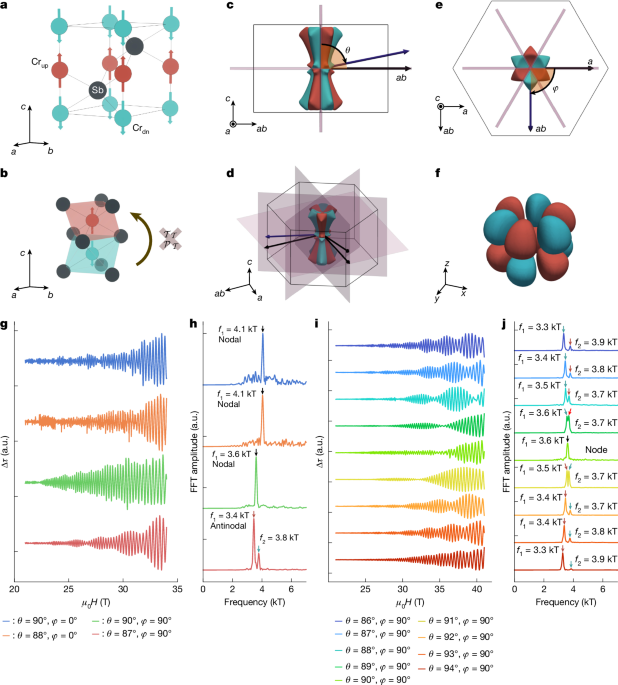
The oscillatory component Δτ was isolated from the background magnetic torque τ by performing a locally estimated scatterplot smoothing (LOESS)⁴⁹ subtraction. In general, owing to the intricate web sheet of the CrSb Fermi surface, the dHvA waveform at a given angle could be quite complicated because of the presence of numerous frequency components. To simplify our analysis and concentrate on the dogbone Fermi sheet, we often performed combined high-pass filtering with short LOESS windows in our analysis. The dogbone frequencies are most prominent above 3 kT, and so we performed Butterworth high-pass filtering of frequencies in inverse field in this range. This was combined with a short sliding LOESS window over τ, which effectively fits any slow oscillations within the background (assumed to be quadratic in H), therefore producing a Δτ waveform dominated by higher-frequency components. For the Δτ traces presented in Fig. 1, this involved using a LOESS window of 0.7 T. In Fig. 2, we used a window of length 1.2 T to show the strong spectral weight at lower frequencies due to the web. By contrast, in Fig. 4, we used a window of only 0.6 T to focus on the >3 kT components in our temperature-dependence study.

DFT calculations

DFT calculations for CrSb were performed using the all-electron, full-potential linearized augmented plane-wave (FP-LAPW) method as implemented in the WIEN2k code⁵⁰. The electronic structure was converged on a 43 × 43 × 28 Monkhorst–Pack k-point mesh within the Brillouin zone of the primitive hexagonal unit cell. Exchange–correlation effects were treated within the generalized gradient approximation. We specified two distinct Cr sites (Cr₁ and Cr₂) within the primitive unit cell, corresponding to Cr atoms adopting up and down spin polarization. Calculations were initialized so that one Cr site has a higher spin-up density and the other has a spin-down density. The onsite spin polarization was then allowed to vary throughout the self-consistency cycles until the compensated collinear ground state was reached. Quantum oscillation frequency analysis of the resultant Fermi surface sheets was determined using SKEAF (ref. ⁵¹). Fermi surface visualization was performed using py_FS (refs. ^48,52).

We assumed that ambient-pressure CrSb in the NiAs-type structure (P6₃/mmc) adopts lattice parameters a = 4.12 Å, b = 4.12 Å and c = 5.47 Å. Within the unit cell, there are two equivalent Cr sites and two equivalent Sb sites, as specified by Extended Data Table 1. We reduce the symmetry of the crystal lattice from P6₃/mmc to P3m1 by specifying that the two Cr sites adopt opposite spins.

DFT calculations converge on a Fermi surface, in which the bands associated with the down and up ‘dogbone’ surfaces are open about the high-symmetry point, corresponding to a cylindrical topology. This is inconsistent with our quantum oscillation measurements, in which we resolve oscillations from these sheets for magnetic fields very close to the a and ab directions. No frequencies would be observed for these field orientations if the sheets were cylindrical. Therefore, we propose that these bands form closed Fermi surface sheets with dogbone-like geometry. To ‘close’ the open Fermi surface sheets of our DFT calculations, we shift our band edges relative to the Fermi energy. The dogbone-like sheets were shifted down by 0.11 eV so that the calculated frequencies along the a, ab and c directions are in good agreement with the quantum oscillation data. As the dogbone sheets are of hole character, we shifted up the ‘web’ sheets (of electron character) by 0.015 eV to keep the total carrier number constant (see Supplementary Information).

Consideration of spin–orbit coupling

Real materials always exhibit some spin–orbit coupling and many-body electronic correlations, meaning a purely non-relativistic framework is only ever an idealization. Nevertheless, our symmetry-based interpretation remains robust. Because CrSb possesses an inversion-symmetric crystal structure, the spatial symmetries protecting the orientation of the nodal planes remain intact. Furthermore, under the intense magnetic fields used in our experiments, field-assisted tunnelling (magnetic breakdown) allows quasiparticles to traverse small hybridization gaps opened by weak spin–orbit coupling, effectively restoring the pristine altermagnetic trajectories. As detailed in the Supplementary Information (in which we also explicitly account for electronic correlations), these considerations justify our simplified symmetry picture introduced here, yielding a direct mapping between the quantum oscillation frequency spectra and the underlying altermagnetic order parameter Δk.

Energy splitting from quantum oscillation frequencies

From the Onsager relation⁴⁵, we can equate a quantum oscillation frequency to a reciprocal space area as

The cyclotron mass of an orbit, m*, is related to the rate of change of the orbital area by

By taking the derivative of equation (1) with respect to E, we then determine

We can use this to determine the energy difference associated with the frequency splitting of two bands:

Spherical harmonic notation

In the text, we represent the symmetry of the altermagnetic spin splitting of CrSb in terms of the real spherical harmonic \({{\mathcal{Y}}}_{4}^{-3}\hspace{0.04pt}(\theta ,\varphi )\).

The complex spherical harmonics can be defined in terms of the associated Legendre polynomials as \({Y}_{{\ell }}^{m}(\theta ,\varphi )={N}_{{\ell }m}{{\rm{e}}}^{{\rm{i}}m\varphi }{P}_{{\ell }}^{m}\hspace{0.03pt}(\cos \theta )\), where N_ℓm is a normalization factor, \({P}_{{\ell }}^{m}(x)\) is an associated Legendre polynomial, and \({Y}_{{\ell }}^{m}(\theta ,\varphi )\) is the complex spherical harmonic for ℓ ≥ 0 and m ∈ [−ℓ, ℓ]. The complex spherical harmonics are eigenfunctions of the total angular momentum operator \({\widehat{L}}^{2}\) and of the generator of rotations about the azimuthal axis \({\widehat{L}}_{z}\), spanning a complete orthonormal basis.

The complex spherical harmonics are defined up to a phase factor e^imφ, and so their magnitude does not change as a function of φ. Therefore, it is convenient to work in the basis of the real spherical harmonics, which have explicit φ dependence, when describing the symmetry of an unconventional magnetic order parameter. We can define the real spherical harmonics \({{\mathcal{Y}}}_{{\ell }}^{m}(\theta ,\varphi )\) in terms of linear combinations of complex harmonics according to

or, equivalently, in terms of the associated Legendre polynomials

Defining the real spherical harmonics this way means they form a complete set that spans the same basis as the complex spherical harmonics; however, importantly, they have well-defined varying magnitudes as a function of φ. This allows us to map the \({{\mathcal{Y}}}_{4}^{-3}\) real spherical harmonic to the g-wave symmetry profile of the altermagnetic order parameter in CrSb.

Contactless resistivity measurements

Contactless resistivity measurements were conducted using the proximity detector oscillator⁵³ technique in pulsed magnetic fields. A selected CrSb sample was mounted on a hand-wound planar coil of 15 turns, acting as the inductive component of the oscillator. The coil diameter was customized to match the sample width for optimal filling factor. A counter-wound outer coil enclosing the same area as the inner coil was added to compensate magnetic flux induced during the field pulse, minimizing background pickup.

As the applied magnetic field is swept, changes in the resistivity ρ and susceptibility χ_s of the sample lead to changes in the inductance of the oscillator and produce a shift in the resonant frequency of the oscillator, which can be described by

where η is the filling factor, d is the sample thickness, and μ_r = 1 + χ_s is the relative magnetic permeability⁵³. For a metallic material such as CrSb, eddy currents restrict the penetration of the radiofrequency field to a characteristic skin depth \(\delta =\sqrt{2\rho /({\mu }_{{\rm{r}}}{\mu }_{0}\omega )}\), where ω is the excitation frequency, such that the frequency response is dominated by changes in the resistivity ρ.

Proximity detector oscillator measurements reported in this study were performed in a 65-T pulsed magnet at the Dresden High Magnetic Field Laboratory in Dresden, Germany, following the methodology in ref. ⁵⁴. A customized ³He cryostat was fitted to the magnet, providing a base temperature of approximately 600 mK throughout the pulses. A raw resonant frequency of 25 MHz was achieved, which was fed into a heterodyne mixing circuit to down-convert the signal to about 10.5 MHz, which was subsequently acquired using a high-definition oscilloscope.

Quantum oscillatory components were analysed over a magnetic field range of 38–63 T using a LOESS background subtraction with an 8-T window and a second-order polynomial background subtraction. A quantum oscillation of frequency 0.8 kT was clearly resolved (Extended Data Fig. 7).

We note that, for sufficiently high magnetic fields, altermagnets have been predicted to exhibit certain distinguishing quantum oscillatory features, such as a distinct frequency splitting at a field-induced Lifshitz transition separating the up and down sheets⁵⁵. However, we measured up to a maximal field strength of 64 T (Extended Data Fig. 7) and observed no such signatures. This is probably due to the very high ordering temperature (and hence energy scale) of altermagnetism in CrSb, which remains robust up to these large field strengths.