Distributed computing

Most calculations in this study were performed on the Triton and Pegasus computing clusters at the Frost Institute for Data Science and Computing at the University of Miami. An overview of our computational pipeline is shown in Extended Data Fig. 3a, indicating the calculation phases that required distributed computing. Except for TM-alig¹³, we developed the algorithms for this study in our laboratory using Python, integrating structural informatics approaches from our previous work^{17,18,19,20,50}. We submitted our compute jobs using the IBM load-sharing facility (LSF) platform and bsub commands wrapped in custom Python scripts.

Downloading the AF2 v.4 dataset

On 20 July 2023, we downloaded the AlphaFold database⁵ to our high-performance computing environment using the protocol provided by the Google-Deepmind GitHub page⁵¹. The download took approximately 1 week, and the compressed archive files (.tar) required 24 tebibytes (TiB) of disk space.

Preparing the AF2 database for distributed computing

The 24 TiB AF2 database contained 1,015,798 single-species archive files (.tar) of various sizes. Using a Python script, we redistributed these files into 607 equally sized 40-gibibyte (GiB) groupings of compressed mmCIF files (.cif.gz). We decompressed the mmCIF files in each 40-GiB grouping using a second Python script and distributed computing. Each 40-gigabyte (GB) grouping contained an average of 353,425 mmCIF files (.cif), occupying an average of 100-GiB on disk. The 607 uncompressed AF2 prediction files occupied collectively 60 TiB on disk. Using a Python script, we next equally distributed the 214,528,851 AF predictions of the 607 groupings into 1,000 job submission files.

Identifying superdark GPCR-like folds

As shown in Extended Data Fig. 3a, we performed an exhaustive search for 7TM folds in the 214,528,851 AF2 predictions using the prototypical GPCR rhodopsin (PDB 1F88, chain A)⁵² as our query structure and the program TM-align¹³. Using the 1,000 job submission files described above, we generated 1,000 tabular output files (TM-align option ‘-outfmt 2’), each containing pairwise alignment results for 214,528,851 AF predictions. We processed this set of 1,000 output files using a Python script, identifying 1,543,898 matches with at least 200 residues and a TM-align score of 0.5. Next, we identified and removed programmatically 82,419 matches corresponding to the obsolete UniProt database⁷ entries as of 1 August 2024, arriving at 1,461,479 AF2 structure matches. Because a TM-align score alone is not a robust metric for matching fold topologies, we had to develop additional structure-based algorithms to rank structural similarity and discern the correct 3D fold topology (Extended Data Fig. 3a).

Aligning hits

To generate and visualize structure-based alignments of related protein models, we developed a two-part Python workflow that automated large-scale pairwise superpositions using TM-align. The first script distributed alignment tasks across the Pegasus computing cluster by dividing the input FASTA file into evenly sized subsets (6,000 sequences per job), creating input directories, and submitting array jobs to the cluster scheduler. Each job invoked a second script, which parsed TM-align output files to extract TM-scores, root mean square deviation values and file paths for each query–target pair. For every pair, the script re-ran TM-align to generate the corresponding 3 × 3 rotation and translation matrices, applied these transformations to the atomic coordinates of the mobile structure and wrote the resulting aligned coordinates to new PDB files labelled by alignment score. This automated system enabled efficient, high-throughput structural superposition and normalization of AlphaFold-predicted models for subsequent comparative analysis and visualization.

Surface-constrained geometric trimming and topology scoring

As outlined in Extended Data Fig. 3a, for each query–hit pair, structures were parsed, preserving residue indices, chain identifiers and atomic coordinates. We then computed a geometric surface representation of the query, yielding a topology-based spatial mask. Using this mask, we cropped the hit model to the subset of residues whose coordinates fall within, or coincide with, the query surface, thereby defining trimming strictly by geometric overlap rather than by sequence span. The trimmed model and the query surface were compared subsequently with quantify coverage over the query surface and summarize topological discrepancies (for example, internal gaps and N-/C-terminal truncations within the overlapped region). These surface-anchored calculations provided the inputs for downstream filtering and ranking of structural hits.

We assign each hit to one of three confidence ranks (r1 > r2 > r3) with a hierarchical decision tree that prioritizes intact, contiguous, high-coverage overlap of the query surface. For every hit we assemble a key comprising coverage, TM-score, hit file and query file, then evaluate three quality gates in order: terminal truncation, coverage gaps and overall coverage. First, if either the N or C terminus is truncated by at least 15% of the overlapped region, the hit cannot be r1. When coverage is at least 0.5 in such cases, the hit is demoted to r2 with a reason flag (–NTC for N-terminal, –CTC for C-terminal); if coverage is less than 0.5 it is classified as r3 with –LC (low coverage). Second, if there are coverage gaps within the overlapped region, we examine their cumulative extent. A cumulative gap of more than 50% forces r3 (–LC), and 15–50% yields r2 (–ICG, incomplete coverage gaps). If gaps are present but small (≤15%), a hit with coverage greater than 0.7 may still qualify as r1 (this is the ‘least stringent’ r1 path under the gaps branch); otherwise it falls to r2 (–ICG). Third, independent of truncation/gap checks, coverage less than 0.7 precludes r1: 0.5–0.7 maps to r2 (–LC) and less than 0.5 maps to r3 (–LC). Hits that clear all three gates—no substantial terminal truncation, no or minimal gaps and coverage of at least 0.7—are assigned r1 by the ‘most stringent’ fall-through path.

Constructing the annotated 7TMP catalogue of hits

As outlined in Extended Data Fig. 3b, we built a master catalogue of sequences and annotations with a four-step Python pipeline, using flat database files for UniProt and InterPro downloaded on 1 September 2025 (offline parsing; no web application programming interfaces). First, raw listings of 7TMP hits were parsed to standardize identifiers (UniProt accession and entry name), capture sequence length and source file paths, normalize heterogeneous headers and remove duplicates, yielding a clean listing table keyed by accession. Second, UniProt flat files (1 September 2025 download) were parsed to extract accession numbers, entry/protein/gene names, organism (and/or TaxID), length and review status, and to harmonize canonical versus isoform records into a metadata table. Third, the listing and UniProt tables were key-merged on accession, preserving provenance paths and adding basic quality control fields (for example, length deltas, missing-metadata flags) to produce a consolidated master table. Finally, InterPro domain annotations from flat files (1 September 2025 download) were integrated by aggregating all protein-to-InterPro mappings per accession and joining them into the master table. The result is a single, analysis-ready CSV/TSV file that unifies cleaned listings, UniProt metadata and InterPro domain sets for downstream filtering, stratification and structural analyses.

GPCR-focused filtering and labelling of 7TMP hits

As outlined in Extended Data Fig. 3b, starting from the annotated catalogue, we applied a two-step rule-based filter to classify 7TMP hits by GPCR status. For each UniProt accession, the script consolidated InterPro signatures and UniProt metadata, then (1) identified GPCR-positive entries using curated GPCR evidence terms and (2) assigned all remaining entries—those not meeting (1)—to a non-GPCR 7TMP set. Results are written as delimited tables and, when enabled, also exported to Excel using a streaming writer suitable for large outputs. This step yields a curated GPCR versus 7TMP partition for downstream analyses.

Surface-trimmed sequence extraction

To convert full-length proteins into sequences that reflect only the geometry retained after surface trimming, we generated gap-aware sequences from the trimmed structural models. For each model, Cα records were traversed in ascending residue number, appending the one-letter amino-acid code only for residues that remained after trimming. Discontinuities in residue numbering or excised segments were encoded as ‘X’ placeholders, preserving registry with the original chain while masking non-overlapping regions. Provenance fields (superkingdom, UniProt accession, gene/protein symbol, organism and rank) were propagated into FASTA headers. For scalability, models were partitioned into balanced chunks and executed as an LSF job array; per chunk FASTA files were then concatenated to yield a single surface-trimmed sequence set for downstream alignment and ranking.

Superkingdom partitioning and priority-preserving sequence clustering

The surface-trimmed sequences set was partitioned by superkingdom from a single FASTA (plain or gzipped) using case-insensitive header classification. For each record, the first token before the first pipe (|) determined assignment to Archaea, Bacteria or Eukaryota; if no match was found, the full header was searched for canonical terms, otherwise the record was labelled Other. Records were streamed to four corresponding FASTA files and a brief count report, using a streaming approach to avoid loading the dataset into memory. We then generated a non-redundant representative set through an incremental, priority-aware MMseqs2 workflow: Archaea sequences were clustered first with linclust (minimum sequence identity 0.50; bidirectional coverage at least 0.50), establishing initial representatives; Bacteria were appended and incorporated with clusterupdate, which projects existing clusters onto the expanded database while preserving current representatives; the same append-and-update step was repeated for Eukaryota. Representatives from the final updated clustering were extracted and exported to FASTA, yielding a compact set that preserves the intended Archaea→Bacteria→Eukaryota priority.

All-versus-all BLASTp on an LSF cluster

Using the representative FASTA produced above, we first created a BLASTp library (protein database) and then performed an all-versus-all BLASTp search by partitioning the FASTA into N whole-record chunks and submitting one job per chunk to the LSF scheduler (bsub). For each chunk, the BLASTp command targeted the newly built database and honoured user parameters (BLOSUM62 or BLOSUM45 with 14/2 gaps, E-value threshold, SEG filtering, xdrop and final xdrop, maximum targets and tabular outfmt 7 fields: qseqid pident length E-value bitscore stitle, with optional per job threads). Outputs were written as one TSV per chunk with corresponding logs, enabling straightforward monitoring and downstream collation of the all-versus-all results.

BLASTp-derived protein similarity network construction

We converted the per chunk BLASTp outputs (tabular outfmt 7) into a compact protein similarity network. BLASTp result lines were streamed, parsing query and subject identifiers from headers formatted as superkingdom|UniProt|gene|organism|rank. One node was created per unique UniProt accession with its associated annotations, and undirected edges were added between protein pairs supported by BLASTp matches. Self-hits were removed, and pair ordering was canonicalized to avoid duplicates. For each protein pair, several hits were aggregated to a single edge by retaining the most informative statistics (for example, maximum percent identity, minimum E-value, maximum bitscore and aligned length. The pipeline writes compressed edge and node tables (including each node’s unique-edge degree) and, optionally, a hits table, yielding an analysis-ready similarity network for downstream visualization and graph analysis.

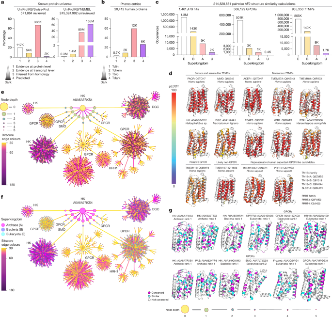
To define meaningful network connections, we applied calibrated similarity thresholds empirically in the BLASTp component. We used bitscore rather than E-value because bitscore is independent of database size, and retained edges with bitscore greater than or equal to 30. This threshold was chosen based on benchmarking against known GPCR relationships in the human GPCRome, which showed that higher cutoffs would exclude many established homologies. We also required at least 30% sequence identity to further minimize spurious links. As shown in Fig. 1g, although BLASTp detects local alignments, the aligned regions were distributed across the 7TM fold rather than confined to short local fragments, supporting broad structural coverage despite local sequence variability. To support reproducibility, we include the benchmarking analysis processed through our pipeline, along with the resulting Cytoscape network and the supplied network file.

Seed-centric traversal of the similarity network

We extracted seed-centred subnetworks from the BLASTp-derived graph using a deterministic go-forward procedure. Starting from the archaeal node with the highest unique-edge degree, candidates were evaluated in a fixed-priority order—higher percent identity, longer aligned length, higher bitscore, lower E-value—with ties resolved by rank (r1 > r2 > r3) and then by a stable identifier. Nodes passing preset quality gates were admitted once (visited-set enforcement), and expansion proceeded layer by layer until no additional qualifying neighbours remained or a predefined node/edge budget was reached. The method outputs Cytoscape-ready node and edge tables, along with summary metrics (subgraph size, degree distribution and threshold provenance).

Strict reduction of the similarity network for Cytoscape

We transformed the BLASTp-derived protein similarity graph into a compact, high-confidence subnetwork suitable for Cytoscape by applying strict, staged reductions. Edge lists were cleaned to remove self-loops and duplicates, canonicalized to a single order per pair, and collapsed to one edge per protein pair by retaining the most informative statistics (for example, highest identity/bitscore, lowest E-value, longest aligned span). Edges were then filtered using stringent similarity gates (identity/bitscore/E-value and coverage), after which connected components were computed and constrained by global and per component node budgets. To control local density and highlight salient relationships, we limited each node to its strongest connections (top-k), enforced a minimum degree and iteratively pruned dangling nodes. The result is a Cytoscape-ready set of tables—reduced edges with summary metrics and reduced nodes with annotations and recomputed degrees—optimized for clear visualization and downstream analysis.

Pairwise alignment and conservation mapping to PDB residue numbering

Pairwise sequence alignments were generated with Clustal Omega, and the alignment ‘traceback’ (symbol) line was parsed to classify each column as identity (*), conservative (:), semi-conservative (.) or gap. For every pair, we reconstructed a column-wise index map from alignment columns to the corresponding ungapped positions in each partner sequence, then translated those sequence positions to PDB residue identifiers (chain, residue number, insertion code) by loading the matching structures (PDB/mmCIF) and building sequence-to-structure mappings. The result was written as a per pair matches table (pos1(PDB) aa1 pos2(PDB) aa2 symbol) that preserves the original PDB residue numbering for both proteins, enabling structure-aware visualization and downstream analyses of conserved sites.

Foldseek structural searches against the afdb50-minimal database

We queried individual protein structures against the prebuilt afdb50-minimal Foldseek database using foldseek easy-search. Before searches, the database prefix was normalized and, if needed, indexed. Runs shared the following settings: alignment type = local 3Di (–alignment-type 0), sensitivity = 9.5 (-s 9.5), coverage = 0.0 with cov-mode = query&target (-c 0.0–cov-mode 0), max-seqs = 10,000 (–max-seqs 10000), iterations = 1 (–num-iterations 1), exhaustive search on (–exhaustive-search), load-on-demand (–db-load-mode 2), threads = 12 (–threads 12) and graphics processing unit off. We then executed two representative calculations that differed only in E-value threshold: a permissive search (E = 1.0) and a stringent search (E = 0.01), producing separate.m8 outputs for downstream parsing.

Automated pocket detection with pHinder

We ran pHinder in virtual screening mode on the AF2 model of TM184C (UniProt Q9NVA4, chain A), with only the virtual-screen branch enabled (virtualScreenSurfacesCalculation = 1; all other calculation toggles = 0). A high-resolution protein surface was computed and saved (circumsphere radius limit 6.5 Å, minimum patch area 10 Ų, high_resolution_surface = 1, save_surface = 1). A sampling grid was laid over the surface with grid_increment = 3.0 Å, sampling points were clash-filtered at 2.5 Å (virtual_clash_cutoff), and the remaining points were connected into a proximity graph with edges less than or equal to 2.0 Å (max_void_network_edge_length). Connected components with fewer than ten points (min_void_network_size) were discarded. For each surviving component, a triangulated void surface was generated and refined with one inward and one outward pass (IN: 1× at 2.0 Å; OUT: 1× at 2.0 Å). Network settings were left at defaults for this step (max_network_edge_length = 10.0 Å, min_network_size = 1, reduced representation and triangulation saving enabled). Hydrogens, waters and ions were excluded; logging was enabled; the Python recursion limit was set to 10,000; and execution used all central processing unit cores minus one. Outputs were written under the specified save path, yielding triangulated, pocket-shaped void surfaces suitable for downstream screening.

Automated pocket detection with Fpocket

Putative ligand-binding pockets were identified with Fpocket, invoked by a lightweight Python wrapper in single-file mode on each PDB structure. The wrapper resolved the Fpocket executable from the system PATH, executed in the parent directory of PDB, captured return codes for provenance and collected results. For our runs, we specified a minimum pocket radius of 3.8 Å (flag -m 3.8); all other Fpocket options were left at their defaults (no condensed/energy modes, no ligand/chain restrictions and no overrides for clustering, distance metrics, α-sphere thresholds or grid settings). This provided reproducible pocket calls suitable for downstream aggregation and analysis.

Upset plots for head-to-head comparison with Foldseek

For our head-to-head comparison with Foldseek, we used the test structures of rhodopsin (PDB 1F88, chain A), β2 adrenergic receptor (PDB 6KR8, chain A), adenosine receptor A2a (PDB 3VG9, chain A) and frizzled (PDB 8QW4, chain A), along with the search parameters described above. Structure-only results were summarized by TM-score and coverage (Extended Data Fig. 4a). For Extended Data Fig. 4b, we took the unique UniProt accessions returned for each query under three conditions—structure-only, Foldseek (E = 1.0), and Foldseek (E = 0.01)—with hits left geometrically unfiltered, constructed a simple membership matrix (IDs × queries) and computed set intersections (Supplementary Data 2). Upset grids display the largest intersections across the four queries (bar heights) alongside per-query totals (left bars), providing a direct, condition-by-condition view of shared versus query-specific hits.

Superdark protein expression

Using tissue- and cell-specific protein expression data downloaded as a flat file (.tsv) from the Human Protein Atlas (v.24, accessed 10 January 2025), we quantified superdark candidate expression patterns using custom Python code. We generated the heat maps in Extended Data Fig. 1a by assigning values of 1, 0.6, 0.3 and 0 to high, medium, low and not detected protein expression levels.

Identifying arrestin codes

Using the built-in Python regular expressions library (re), we compiled regular expression patterns for short (r”[ST].[ST][^P][^P][STED]”) and long (r”[ST]..[ST][^P][^P][STED]”) arrestin codes. We then searched each superdark sequence for these string patterns, limiting our analysis to the C terminus as predicted in each AF2 model. All protein sequences were downloaded using the UniProt application programming interface in FASTA format.

Identifying lysosome di-leucine motif codes

We used the same procedure for finding arrestin codes, but we used a compiled regular expression pattern for di_leucine motifs (r”[DE]…L[LI]”).

Software used

The following software was used: Conda (v.24.9.2), Python (v.3.8.17), Biopython (v.1.78), TM-align (v.20210224), Foldseek (v.10.941cd33), BLASTp (v.2.26.0+), Clustal Omega (v.1.2.4), pHinder (v.7.0), Fpocket (v.4.1), MMseqs2 (v.18.8cc5c), Cytoscape (v.3.10.3) and PyMOL (v.3.4.19).

Cell culture

HEK293T and SK-MEL-28 cells were obtained from the American Type Culture Collection. HEK293A cells were obtained from Asuka Inoue—a base strain originally from Thermo Fisher. HEK293T and HEK293A cells were maintained in DMEM medium (Gibco) supplemented with 10% FBS and 1% penicillin–streptomycin. SK-MEL-28 cells were cultured in RPMI-1640 medium (Gibco) with 10% FBS and 1% penicillin–streptomycin. The hTERT human adult astrocytes were obtained from the Bayik laboratory (originally from University of California, San Francisco) and maintained in DMEM F12 with Glutagro (Corning), N-2 supplement (Thermo fisher), human epidermal growth factor (EGF) (PeproTech) 20 ng ml⁻¹, human fibroblast growth factor (FGF) (PeproTech) 20 ng ml⁻¹, 5% FBS, 1% penicillin–streptomycin. L1 cell line with mito-mCherry (from the Bayik laboratory) was maintained in DMEM F12 with Glutagro, B-27 supplement (Thermo fisher), EGF 20 ng ml⁻¹, FGF 20 ng ml⁻¹ and 1% penicillin–streptomycin. The primary GBM cell line (from the Ivan laboratory) was maintained in DMEM F12 with Glutagro, N-2 supplement, B-27 supplement, EGF 20 ng ml⁻¹, FGF 20 ng ml⁻¹, 1 mM sodium pyruvate, 2 μg ml⁻¹ heparin (Sigma) and 1% penicillin–streptomycin in a flask with 5 μg cm⁻² fibronectin (Corning). All cells were cultured in a humidified incubator at 37 °C with 5% CO₂. The passage number was recorded for each cell line.

Lentivirus production

Lentiviral particles were generated using HEK293T cells. Cells were seeded at a density determined by the size of the dish or plate in DMEM containing 10% FBS and 1% penicillin/streptomycin. After overnight incubation, cells were transfected using PolyJet (SignaGen Laboratories) at a 1:3.33 plasmid:PolyJet ratio, with a plasmid mixture containing a 4:3:1 ratio of transfer:Δ8.2:vsv-g plasmids. Approximately 48 h after transfection, culture media were collected and replaced with fresh media. Viral supernatant was collected on days 2 and 3 following transfection. The collected supernatants were combined and filtered through a 0.45-μm mixed cellulose esters filter (Millipore) to remove cellular debris, and the filtrate was stored at −80 °C until further use.

Stable cell line generation using lentiviral transduction for imaging

All stable cell lines with TM184A, TM184B and TM184C full-length and mutants tagged with eGFP or mCherry were generated for each cell line in the same way, except each had the appropriate concentration of puromycin (HEK293A, SK-MEL-28, HFF-1, primary GBM cell line = 1 μg ml⁻¹). Cells were seeded at 50–70% confluency per well in a six-well plate. The following day, cells were infected with filtered lentiviral particles. After 24 h, the virus-containing medium was removed and replaced with fresh medium. The next day, cells were split, maintaining a confluence of 80–100%, and, appropriate to the cell line, the medium was added. There was always a non-transduced control for selection to ensure the puromycin concentration was kept at the lowest possible level. After the cells recovered, they were further split into larger dishes and maintained at 80–100% confluence. The hTERT human astrocytes and L1 mito-mCherry PDX cell line were selected using fluorescence-activated cell sorting (FACS) on a BD FACSAria II (BD Biosciences) with FACSDiva software instead of puromycin. In brief, either the TM184C–eGFP-positive or the double-positive population of L1 mito-mCherry and TM184C–eGFP was sorted into 12-well or 24-well dishes (Supplementary Fig. 2). All stable cell lines were maintained as polyclonal populations at the appropriate puromycin concentration. HEK293T and SK-MEL-28 cells (American Type Culture Collection) are authenticated by the vendor at source; the HEK293A, HFF-1, hTERT-immortalized astrocyte and patient-derived (L1 xenograft and primary GBM) lines were not re-authenticated independently by short tandem repeat profiling. All cell lines tested negative for mycoplasma contamination by PCR. None of the lines used (HEK293T, HEK293A, SK-MEL-28, HFF-1, hTERT astrocytes, L1, primary GBM) appear on the ICLAC Register of Commonly Misidentified Cell Lines.

For co-localization experiments, the stable cell lines with full-length or mutant TM184C tagged with eGFP or mCherry were seeded in confocal dishes to reach 30–50% confluency the next day. For imaging astrocytes and primary GBM cell lines, the plates were coated additionally with 5 μg ml⁻¹ fibronectin for 30–60 min. Then these were transfected with TransiT-2020 (3 μl:1 μg of plasmid) and 1 μg of the indicated plasmid, each tagged with mVenus, mCherry, mRFP1 or YFP. The cells were imaged 24–48 h after transfection, and treatments with autophagy modulators (‘Autophagic flux’) were performed for the indicated time period and dosage, coinciding with the day of imaging.

Plasmids

ARRB1- and ARRB2-Venus were gifts from K. D. G. Pfleger. We took arestin1 and 2 to create 3xHA–ARRB1 and 3xHA–ARRB2. The plasmids containing all mini G, 4AG alpha and bystander markers with mVenus or RLuc8 were gifts from N. Lambert. pLJM1–eGFP, pLJM1-LAMP1-mRFP1-FLAG, pcDNA3.1-mCherry-hLC3B, lentiCRISPR-v2, lentiCRISPR-v2 blast, mCherry-ActA-IRES-puromycin-pLVx-EF1a, TRUPATH plasmid kit and PRESTO-Tango plasmid kit were all obtained from Addgene.

pcDNA3.1(+)-Superdark constructs were generated using HiFi DNA assembly (New England Biolabs). Superdark genes were codon-optimized for humans (GeneScript), then obtained as gBlocks (Integrated DNA Technologies) and amplified by PCR using primers designed to overlap with the pcDNA3.1(+) backbone and the start and stop codons of each superdark sequence. Backbone and insert constructs were co-incubated with HiFi master mix and transformed into competent DH5α Escherichia coli.

The pcDNA3.1(+)-Superdark-RLuc8 constructs were generated using HiFi DNA assembly. The linker (GVPRARDPPVAT) and RLuc8 tag were amplified from GPR4-RLuc8 (gift from N. Lambert), using primers that provided homology to the C-terminal tails of the superdark constructs and pcDNA backbone. The backbone with superdark gene and RLuc8 insert constructs were co-incubated with HiFi master mix and transformed into competent DH5α cells to form fully intact plasmids.

For adding or changing small DNA sequences (HiBiT and HA tags, point mutations, gRNA sequences), the same strategy, called 5’-phosphate PCR assembly, was used. Briefly, vectors were amplified using Q5 High-Fidelity DNA Polymerase (NEB) reactions with a 5’-phosphate-modified complementary primer, a primer containing the desired change, a complementary region (in opposite orientations) and the template plasmid DNA. PCR products were verified by agarose gel electrophoresis, then digested with DpnI (NEB) at 37 °C for 1.5 h, followed by heat inactivation. Ligation was performed overnight at 16 °C or for 2 h at room temperature using T4 DNA ligase (NEB). Ligase was heat-inactivated, and 2 µl of the ligation mix was transformed into competent DH5α cells.

All plasmids were verified by Sanger or nanopore sequencing (Eurofins Genomics).

CRISPR–Cas9-mediated genome editing

Plasmids

Plasmids were constructed using the above 5′-phosphate PCR assembly strategy. Six gRNA sequences targeting the TM184C mRNA were selected and screened for optimal efficiency. Two of the six gRNA sequences are used and shown in the study.

Transient transfection in HEK

HEK293T cells were seeded at 300,000 cells per well in six-well plates. After 24 h, cells were transfected transiently with 1.25 μg of plasmid DNA and 3 μl μg⁻¹ of POLYJET in Advanced DMEM (Gibco). After 24–48 h, the cells were trypsinized and resuspended in medium containing puromycin at 1 μg ml⁻¹. Cells were split into the desired-sized plate or dish. There was always a non-transfected control for the selection to ensure the puromycin selection agent was working as expected. Once the controls were dead, the experimental cells were then collected for analysis.

Rescue experiments

Because TM184C behaved as an essential gene, the established stable cell lines with full-length or mutant TM184C tagged with eGFP or mCherry, and parental HEK293A cells, were used as the base cells. The stably integrated GFP-tagged transgenes are codon-optimized and therefore resistant to the endogenous TM184C-targeting gRNAs. In brief, they were transfected with lentiCRISPR-v2 blast plasmids with corresponding gRNAs targeting TM184C, then selected with puromycin at 1 μg ml⁻¹ and blasticidin at 10 μg ml⁻¹.

HiBiT LgBiT assay

HEK293T cells were seeded at 300,000 cells per well in six-well plates. After 24 h, cells were transfected transiently with 1 μg of N-terminal tagged HiBiT receptor, 3 μl of TransIT-2020 (Mirus) transfection reagent per microgram of DNA and 100 μl of advanced DMEM (ADMEM). Control samples were transfected with empty vector. Cells were washed with PBS as described in the bystander BRET protocol and resuspended before transferring 30 μl into a 384-well plate in quadruplicate. A 1:100 dilution of LgBiT and a 1:50 dilution of substrate solution (Promega, Nano-Glo HiBiT Extracellular Detection Kit) were prepared and mixed. A 30-μl aliquot of this mixture was transferred to a 384-well plate, and luminescence was measured after a 10-min incubation using a ClarioStar plate reader. Emission was read at 450-25, gain 3,600, with a measurement interval time of 0.10 s.

Bystander BRET assay

HEK293T cells were seeded at 300,000 cells per well in six-well plates. After 24 h, cells were transfected transiently with 200 ng of RLuc8-tagged receptor, 1 μg of mVenus-labelled bystander protein or empty vector for RLuc8 control, and 3 μl of TransIT-2020 (Mirus) per microgram of DNA in 120 μl of ADMEM. After 48 h, the medium was aspirated, and the cells were resuspended in 1 ml of PBS. A 300-μl aliquot was transferred to a 96-well plate and centrifuged at 300 relative centrifugal force (RCF) for 3 min. The supernatant was aspirated, and 150 μl of fresh PBS was added, followed by gentle resuspension of the pellet. A 30-μl aliquot of the cell suspension was transferred into a 384-well white-bottom plate in quadruplicate. Coelenterazine-h (Nanolight Technology) was added at a final concentration of 5 μM for a total volume of 45 μl. The plate was vortexed for 15 s at 1,750 rpm before luminescence readings were taken using a ClarioStar plate reader in multichromatic mode, with emissions 532.5-25 and 485-20, gain 3,600 and a measurement interval time of 1 s. Emission intensities for RLuc8 and Venus were recorded, and the net BRET ratio was calculated by subtracting the RLuc8–Venus ratio from the RLuc8 control.

4AG protein recruitment assay

For 4AG protein coupling, HEK293T cells were seeded at 300,000 cells per well in six-well plates. After 24 h, cells were transfected with Receptor–RLuc8, 4A subunit, Venus-1–155-Gγ₂, Venus-155–239-Gβ₁ and pcDNA3.1(+) in a (1:10:5:5:5) ratio for a total of 2.6 μg of plasmid DNA and 3 µl µg⁻¹ TransIT-2020 (Mirus) in each well of a six-well plate. After a 24–48-h incubation following transfection, the plates were aspirated, cells were washed, resuspended and 30 μl was added to a 384-well plate in quadruplicate, as in the bystander BRET protocol. Coelenterazine-h was then added at a 5 μM final concentration for a final volume of 45 µl. The plate was then read using the ClarioStar settings from Bystander BRET.

TRUPATH G-protein dissociation assay

HEK293T cells were seeded at 300,000 cells per well in six-well plates. After 24 h, cells were transfected transiently using a 1:1:1:1 DNA ratio of receptor: Gα–RLuc8:Gβ:Gγ–GFP2 (100 ng per construct for six-well dishes). TransIT-2020 (Mirus) was used to complex the DNA at a ratio of 3 µl TransIT DNA per microgram DNA in ADMEM. At 48 h after transfection, the plates were aspirated, cells were washed, resuspended and 30 μl was added to a 384-well plate in quadruplicate, as in the bystander BRET protocol. Prolume Purple (Nanolight Technology) was then added to a final concentration of 5 μM, resulting in a final volume of 45 µl. The plate was then read on the ClarioStar in multichromatic mode at emissions 400-10 and 520-10, with a 3,600 gain, spiral average, 2-mm diameter and a 0.27 s measurement interval. The same process was repeated, but with varying receptor concentrations to increase constitutive activity through G_s dissociation compared with DRD2.

β-Arrestin-BRET recruitment assay

HEK293T cells were seeded at 300,000 cells per well in six-well plates. After 24 h, cells were transfected transiently with a 1:10 ratio of receptor-RLuc8: Arrestin-mVenus (1.1 μg total DNA), using 3 μl of TransIT-2020 (Mirus) transfection reagent per microgram of DNA in 160 μl of ADMEM. After 48 h, the protocol was identical to the bystander BRET assay described above. The plate was then read using the ClarioStar settings from Bystander BRET.

β-Arrestin-BRET and GRK recruitment assay

HEK293T cells were seeded at 300,000 cells per well in six-well plates. After 24 h, cells were transfected transiently with a 1:5:10 ratio of receptor-RLuc8: GRK (2,3,5,6) or empty vector: Arrestin-mVenus (1.6 μg total DNA) using 3 μl of TransIT-2020 (Mirus) transfection reagent per microgram of DNA in 160 μl of ADMEM. After 48 h, the protocol was identical to the bystander BRET assay described above. The plate was then read using the ClarioStar settings from Bystander BRET.

GRK2 recruitment assay

HEK293T cells were seeded at 300,000 cells per well in six-well plates. After 24 h, cells were transfected transiently with a 1:10 ratio of receptor-RLuc8: GRK2-mVenus (1.1 μg total DNA), using 3 μl of TransIT-2020 (Mirus) transfection reagent per microgram of DNA in 160 μl of ADMEM. After 48 h, the protocol was identical to the bystander BRET assay described above. The plate was then read using the ClarioStar settings from Bystander BRET.

Immunoprecipitation

HEK293 T cells were seeded at 3 million cells in a 10-cm plate. The following day, cells were transfected transiently with 4 μg of DNA for single endogenous IPs, 2 μg:2 μg for two-construct Co-IPs or 3 μg:1 μg for Co-IP with receptors and β-arrestins, using 3 μl of TransIT transfection reagent per microgram of DNA in 400 μl of ADMEM. After 48 h, the medium was aspirated, and cells were washed with cold PBS and centrifuged at 1,000 RCF for 5 min. The PBS was aspirated, and cells were lysed using lysis buffer containing 20 mM HEPES, pH 7.5, 100 mM NaCl, 1 mM EDTA, 1 mM phenylmethylsulfonyl fluoride (PMSF), 1× EDTA-free protease inhibitor cocktail (Sigma), 1 mM MgCl₂, 10 mM β-glycerophosphate (Sigma), 10 mM sodium pyrophosphate (Sigma) and 1% Triton X-100 (Sigma). Lysis was performed for 30 min with vortexing every 5 min. The lysate was centrifuged at 14,000 RCF for 10 min; 500 μl of the supernatant was combined with 10 μg of anti-FLAG M2 antibody (Sigma, catalogue no. F1804) or anti-HA.11 antibody (Biolegend, catalogue no. 901502) and incubated for 1–2 h or overnight at 4 °C with end-over-end mixing.

Pierce Protein A/G Magnetic Beads (0.25 mg; Thermo Fisher) were added to a 1.5-ml microcentrifuge tube for immunoprecipitation. Beads were washed with 175 μl of Wash Buffer (TBS, 0.05% Tween-20 and 0.15 M NaCl) and vortexed gently before collecting using a magnetic stand; the supernatant was discarded. The beads were washed three times with the wash buffer. The antigen–antibody mixture was then added to the beads and incubated at room temperature for 1 h with gentle mixing. The beads were collected using a magnetic stand and washed twice with 500 μl of wash buffer, then washed a final time with 500 μl of purified water. The beads were collected on a magnetic stand and the supernatant was discarded.

For elution, 50 μl of low-pH elution buffer (0.1 M glycine, pH 2.0) was added, and the beads were incubated at room temperature with mixing at 1,400 rpm for 10 min. Beads were collected using a magnetic stand, and the supernatant was transferred to a new tube containing 7.5 μl of neutralization buffer (1 M Tris, pH 9.0) per 50 μl of eluate. The final samples were analysed using SDS–PAGE and western blot.

Immunoblotting from cell lines

Cells were disrupted on ice using the same lysis buffer as the one above. The resulting lysates underwent centrifugation to remove cellular debris, and protein concentrations were quantified using the BCA Protein Assay (Thermo Fisher Scientific). Samples were then separated by electrophoresis and transferred onto 0.22-μm polyvinylidene fluoride membranes (GenScript). The membranes were blocked in Tris-buffered saline Tween (TBST) containing 5% milk (ApexBio) before incubation with the following primary antibodies: Histone H3 (Cell Signaling Technology (CST), catalogue no. 12648), FLAG M2 (Sigma, catalogue no. F1804), TM184C (Atlas Antibodies, catalogue no. HPA054013), LC3B (CST Autophagy Atg8 Family Antibody Sampler Kit, catalogue no. 64459) and VDAC1/Porin (Abcam, catalogue no. ab110326, clone 16G9E6BC4; yeast loading control). Following washes in TBST, membranes were incubated with the following secondary antibodies: anti-rabbit IgG HRP conjugate (Cytiva, catalogue no. NA934) and anti-mouse IgG HRP conjugate (Cytiva, catalogue no. NA931). After further washes with TBST, protein bands were visualized through chemiluminescence using Clarity Western ECL substrate (Bio-Rad) or diluted SuperSignal West Atto substrates (Thermo Fisher Scientific). The densitometric analysis of the blots was performed using ImageJ. Fold changes in expression levels of the construct were analysed relative to the corresponding control signals.

Immunoblotting from yeast

Yeast cells were grown overnight in YPD medium. Cells equivalent to an optical density (OD)₆₀₀ of 1.2 were collected by centrifugation (6,000 RCF, 1 min) and washed with sterile water. The cell pellet was resuspended in 75 µl of Rodel Mix (0.37 M NaOH, 8.9% v/v β-mercaptoethanol, and 10 mM PMSF added fresh), then 500 µl of sterile water was added. After vortexing, an equal volume of 50% trichloroacetic acid was added. The mixture was incubated on ice for 10–15 min and centrifuged (14,000 RCF, 4 °C, 10 min). The supernatant was discarded, and the pellet washed sequentially with 500 µl of 0.5 M Tris base (unadjusted pH) and 500 µl of sterile water (14,000 RCF, 4 °C, 5 min) without disturbing the pellet. The final pellet was resuspended in 25 µl of resuspension buffer (100 mM NaCl, 20 mM HEPES, pH 7.4, 1 mM EDTA, 1 mM fresh PMSF), and the protein concentration was measured by BCA assay. The SDS sample buffer was loaded onto the SDS–PAGE gel for further analysis.

Autophagic flux

To measure autophagic flux upon knockdown of TM184C, the CRISPR-edited HEK293T cells selected with puromycin (see ‘CRISPR–Cas9-mediated genome editing’) were treated with 1 nM of Concanamycin A (Cayman Chemicals) or vehicle (0.06% acetonitrile final) for 24 h. The cells were then processed for LC3B immunoblotting. For imaging, Concanamycin A or Bafilomycin A1 (CST) at 1 nM was used for 18–24 h, as indicated in the legends.

Protein expression and purification

HEK293T cells expressing FLAG-tagged TM184C were collected by scraping, washed with cold PBS, then centrifuged and flash-frozen in liquid nitrogen. For membrane preparation, thawed cells were homogenized in low-salt buffer (10 mM HEPES, pH 7.5, 10 mM MgCl₂, 20 mM KCl) supplemented with protease inhibitors (Roche). The homogenate was incubated for 15 min at room temperature with benzonase (Millipore) and MgCl₂ to a final concentration of 2.5 mM. Following homogenization, cell lysates were subjected to ultracentrifugation at 105,000 RCF for 40 min at 4 °C to isolate membranes. This was repeated twice with a high-salt buffer (10 mM HEPES, pH 7.5, 10 mM MgCl₂, 20 mM KCl, 1 M NaCl) supplemented with protease inhibitors, and the membranes were then ready for downstream purification. They were solubilized in 1%/0.2% dodecyl-β-d-maltoside (DDM)/ cholesteryl hemisuccinate (CHS) (Anatrace) HNG buffer (20 mM HEPES pH 7.5, 300 mM NaCl, 10% glycerol) with 1 mM EDTA for 3 h with rotation at 4°C, clarified by ultracentrifugation at 105,000 RCF for 40 min at 4 °C, then incubated with washed anti-FLAG M2 resin (Sigma) overnight. The beads were then collected in a column and washed three times with ten column volumes of 0.1%/0.02%, 0.05%/0.025% and 0.025%/0.0125% DDM/CHS HNG buffer. FLAG–TM184C was eluted in flag elution buffer (300 mM NaCl, HNG buffer 1 mM EDTA, 0.025%/0.0125% DDM/CHS + 200 μg ml⁻¹ FLAG peptide). The eluates were then concentrated in a Vivaspin 500 (Cytiva) with a 100,000 molecular weight cut-off and loaded onto an SDS–PAGE gel for further analysis. All buffers were prepared with 0.22-µm-filtered reagents, and all steps were performed at 4°C or on ice.

Lambda phosphatase treatment of cell lysates

HEK293T lysates expressing FLAG–TM184C and empty vector, GRK2, GRK3, GRK5 and GRK6 were prepared using a lysis buffer consisting of 20 mM HEPES pH 7.5, 100 mM NaCl, 1 mM EDTA, 1% Triton X-100, 1× protease inhibitor cocktail and 1 mM PMSF. Following a 20-min incubation on ice, lysates were centrifuged at 14,000 RCF for 10 min. A 50 µl aliquot of the supernatant was transferred to a PCR tube and 5 µl of 10× MnCl₂ (NEB) was added, followed by 2.5 µl of lambda phosphatase (NEB). The reaction was incubated at 30 °C for 1 h. The addition of SDS sample buffer terminated the reaction, and samples were incubated at room temperature for 5 min before loading onto a gel for further analysis.

Yeast strains

Yeast strains were maintained and grown in a YPD medium composed of 1 g l⁻¹ yeast extract, 2 g l⁻¹ peptone and 20 g l⁻¹ dextrose. Synthetic complete medium (SCM) is composed of 1.7 g l⁻¹ yeast nitrogen base without amino acids and ammonium sulfate, 20 g l⁻¹ dextrose, 5 g l⁻¹ ammonium sulfate, 20 g l⁻¹ d-glucose and the recommended amount of complete supplement mixture—complete or without uracil powder (MP Biomedicals).

gRNA plasmid and hfl1Δ strain generation

A CRISPR gRNA plasmid targeting HFL1 (pML104-HFL1.1031) was constructed in the pML104 vector using the 5’ phosphate PCR assembly. A 100-bp repair DNA payload for hfl1Δ was created by annealing complementary 50-bp homology arm oligonucleotides designed to flank the HFL1 coding region. Annealing was verified by agarose gel electrophoresis. S. cerevisiae BY4741 strains containing a pre-integrated X-2 landing pad (BY4741 X-2 LP) were transformed with pML104-HFL1.1031 and the repair DNA payload using a standard lithium acetate/polyethylene glycol method. The hfl1Δ yeast strain was verified by the following method. Yeast gDNA was extracted from transformants and PCR was performed using primers flanking the HFL1 coding region. hfl1Δ deletion was confirmed by agarose gel electrophoresis based on PCR product size. Verified hfl1Δ strains were counter-selected on 5-fluoroorotic acid plates to remove the CRISPR plasmid.

Superdark protein integration into hfl1Δ X-2 LP strains

For integration of superdark proteins (TM184A, TM184B, TM184C) or HFL1 into the X-2 LP of hfl1Δ strains, a PCR-generated DNA payload containing superdark protein sequences or the HFL1 gene and X-2 LP homology arms using either the pcDNA3.1 plasmids or the yeast genome as a template. hfl1Δ strains were transformed with pML104-X2 gRNA plasmid (targeting the X-2 LP) and the DNA payload using the same lithium acetate/polyethylene glycol method as above.

FM4-64 staining of yeast vacuoles

Strains were grown in SCM overnight at 30 °C with shaking. The following day, yeast cells were diluted to an OD = 0.2 in 5 ml of SCM and grown in a shaking incubator at 30 °C for around 36–40 h, reaching saturation. Finally, yeast cells were set to an OD of 1.0 in fresh SCM for confocal analysis. A 1-ml aliquot of yeast cells, normalized to an OD of 1.0, was transferred to a 1.5-ml sterile Eppendorf tube and centrifuged at 10,000 RCF for 3 min. The supernatant was removed, and yeast cells were resuspended in 100 μl of fresh SCM. Then, 3 μl of 1 mM FM4-64 dye was added to the sample, vortexed and incubated at 30 °C (no shaking) for 20 min (final FM4-64 dye concentration around 29.1 μM). Cells were centrifuged at 10,000 RCF for 3 min, and the supernatant was discarded. Yeast cells were washed with 100 μl of fresh SCM, centrifuged at 10,000 RCF for 3 min and the supernatant was discarded. This process was repeated for a total of two washes. Yeast cells were resuspended in 200 μl of fresh SCM before 6 μl of the yeast mixture was plated on a 2% SCM agarose pad, and a glass coverslip was dropped onto the agarose pad.

MS data acquisition and analysis from on-bead digestion

Two immunoprecipitation samples were subjected to on-bead tryptic digestion according to an established protocol⁵³. Bead-bound proteins were digested by adding 10 µl of trypsin (10 ng µl⁻¹) in 100 mM ammonium bicarbonate (AMBIC) at an enzyme-to-protein ratio of 1:100 (wt/wt). Beads were vortexed every 2–3 min for the first 15 min to ensure homogeneous protease distribution, then incubated overnight at 37 °C. A second aliquot of trypsin was added the following day for an additional 4-h digestion at 37 °C. Supernatants were collected using a magnetic rack, acidified to 5% formic acid (v/v), and desalted using C18 ultra micro spin columns per the manufacturer’s instructions. Samples were dried by vacuum centrifugation and reconstituted in 1% acetic acid before analysis.

Peptides were separated and analysed on a ThermoScientific Fusion Lumos Tribrid mass spectrometer coupled to a Dionex Ultimate 3000 RSLCnano HPLC system. Each sample (5 µl) was loaded onto an Acclaim PepMap C18 trapping column (100 µm × 2 cm, 5 µm, 100 Å), then resolved on an Acclaim PepMap C18 analytical column (75 µm × 25 cm, 2 µm, 100 Å) using a 140-min gradient from 2% to 90% acetonitrile in 0.1% formic acid at 0.3 µl min⁻¹. The microelectrospray ion source was operated at 2.5 kV. Data-dependent acquisition was performed with a 3-s duty cycle: full MS1 scans were acquired at a resolution of 120,000 over m/z 350–1,500 (automatic gain control target 4.0 × 10⁵), followed by MS2 fragmentation using collision-induced dissociation (35% collision energy, 1.6 Da isolation window, ion trap detection, automatic gain control 2.0 × 10³). Dynamic exclusion was applied for 60 s within a 10 ppm window after one repeat.

Raw data were searched against the human SwissProtKB database (26,576 entries, downloaded March 2022) using Sequest within Proteome Discoverer v.2.5. Search parameters included full tryptic cleavage with up to two missed cleavages, 10 ppm MS1 and 0.06 Da MS2 mass tolerances, variable oxidation of methionine and N-terminal acetylation, and static carbamidomethylation of cysteine. Peptide and protein identifications were validated using Percolator with a reverse-decoy strategy, requiring at least two peptides per protein and a false discovery rate less than or equal to 1% at both the peptide and protein levels. To investigate post-translational modifications, the dataset was also queried against the TM184C sequence with phosphorylation included as a variable modification, yielding three phosphopeptides with distinct phosphorylation sites mapping to serine residues S422, S432 and S435.

MS data acquisition and analysis from gel

Purified TM184C was loaded onto an SDS–polyacrylamide gel and stained with a Coomassie dye. The band indicated in the figure was cut to minimize excess polyacrylamide and divided into several smaller pieces for protein digestion. The gel pieces were washed with water and dehydrated in acetonitrile. The bands were then reduced with dithiothreitol and alkylated with iodoacetamide before the in-gel digestion. All bands were digested in-gel using trypsin by adding 5 μl 10 ng μl⁻¹ trypsin or chymotrypsin in 50 mM ammonium bicarbonate and incubating overnight at room temperature to achieve complete digestion. The peptides formed were extracted from the polyacrylamide in two aliquots of 30 µl each, using 50% acetonitrile with 5% formic acid. These extracts were combined and evaporated to less than 10 μl in a Speedvac, then resuspended in 1% acetic acid to a final volume of approximately 30 μl for liquid chromatography–mass spectrometry analysis.

The liquid chromatography–mass spectrometry system was a Bruker TimsTof Pro2 Q-Tof mass spectrometer operating in positive-ion mode, coupled with a CaptiveSpray ion source (Bruker Daltonik GmbH). The HPLC column was a Bruker 15 cm × 75 µm id C18 ReproSil AQ, 1.9 μm, 120 Å reversed-phase capillary chromatography column. Extract (1 μl) was injected, and the peptides eluted from the column by an acetonitrile/0.1% formic acid gradient at a flow rate of 0.3 μl min⁻¹ were introduced into the mass spectrometer source online. The digests were analysed using a parallel accumulation serial fragmentation DDA method to select precursor ions for fragmentation with a trapped ion mobility–mass spectrometry scan followed by ten parallel accumulation serial fragmentation tandem mass spectrometry scans. The trapped ion mobility–mass spectrometry survey scan was acquired over 0.60–1.6 V cm⁻² and 100–1,700 m/z, with a ramp time of 166 ms. The total cycle time for the parallel accumulation serial fragmentation scans was 1.2 s, and the tandem mass spectrometry experiments were performed with collision energies between 20 eV (0.6 V cm⁻²) and 59 eV (1.6 V cm⁻²). Precursors with two to five charges were selected with the target value set to 20,000 a.u. and an intensity threshold of 2,500 a.u. Precursors were dynamically excluded for 0.4 s.

Data were analysed using all collision-induced dissociation spectra collected in the experiment to search the human SwissProt database using the program MSFragger. These samples were analysed using a low-coverage gradient from 2% to 70% acetonitrile over 110 min.

Confocal microscopy

Microscopy was performed using a Leica Stellaris 5 confocal inverted microscope equipped with a ×63 oil-immersion objective lens and operated by Leica Application Suite X software (LAS X; v1.4.6.28433). Image acquisition was performed by a line-scan. The Leica LAS X Dye Assistant module was used to obtain optimal spectral yield and minimal overlap. The acquisition format was 1,024 × 1,024, speed 400–700, bidirectional X and pinhole at Airy 1. The four HyD detectors were set to analogue or counting mode with 16-bit depth for vesicle transfer and immunofluorescence experiments. All mammalian cells were seeded onto 35-mm confocal dishes with 20-mm glass bottoms (VWR, catalogue no. 75856-742) or in Nunc 27 mm glass-bottom dishes (Thermo Fisher Scientific, catalogue no. 150682) and cultured for 24 h or 48 h under standard conditions (37 °C, 5% CO₂). For immunofluorescence, the same dishes and culture conditions were used, followed by standard fixation and the antibody protocol described in ‘Fixed-cell immunofluorescence microscopy sample preparation’. For fixed mammalian cell samples, images consisted of z-stacks determined by the Leica LAS X System Optimized Z sectional thickness. For live-cell mammalian imaging experiments, three to five optical sections per z-stack were acquired, using the time interval minimize feature.

Fixed-cell immunofluorescence microscopy sample preparation

For immunofluorescence microscopy, cells were fixed in 4% paraformaldehyde for 10 min at room temperature, followed by three 5-min washes in PBS. Cells were permeabilized using 0.1% Triton X-100 in PBS for 10 min, followed by an additional PBS wash. Blocking was performed with 1% bovine serum albumin in PBS for 1 h at room temperature. Primary antibody incubation was carried out using rabbit anti-human TM184C antibody (Thomas Scientific, catalogue no. HPA054013-100) on wild-type HEK293A cells. For TM184C–eGFP fusion stable line immunofluorescence, KIF5B (CST, catalogue no. 62696) primary antibody was used. All antibodies were diluted in blocking buffer overnight (12 h) at 4 °C. After three PBS washes, cells were incubated with goat anti-rabbit IgG conjugated to Alexa Fluor 647 (CST, catalogue no. 4414S) for 1 h at room temperature. Following final PBS washes, samples were mounted using ProLong Diamond Antifade Mountant containing DAPI (Thermo Fisher Scientific, catalogue no. P36962).

Live-cell microscopy

All mammalian cells were seeded onto 35-mm confocal dishes with 20 mm glass bottoms (VWR, catalogue no. 75856-742) or in Nunc 27 mm glass-bottom dishes (Thermo Fisher Scientific, catalogue no. 150682) and cultured for 24 h or 48 h. For live-cell imaging, the culture medium was replaced with FluoroBrite DMEM (Thermo Fisher Scientific, catalogue no. A1896701). Depending on the experimental conditions, cells were treated with one or more of the following fluorescent markers: NucBlue Live ReadyProbes Reagent (Thermo Fisher Scientific, catalogue no. R37605), Tubulin Tracker Deep Red (Thermo Fisher Scientific, catalogue no. T34076) or LysoTracker Red DND-99 (Thermo Fisher Scientific, catalogue no. L7528). Each dye was incubated for 15 min, followed by exchange into fresh FluoroBrite DMEM.

Imaging of yeast vacuoles

Yeast vacuoles were stained using FM4-64 dye (Thermo Fisher Scientific). FM4-64 powder was dissolved in nuclease-free water to a stock concentration of 1 mM and stored in aliquots protected from light at −20 °C. For staining, yeast cells normalized to OD₆₀₀ = 1.0 were pelleted by centrifugation at 10,000g for 3 min and resuspended in 100 μl fresh SCM containing FM4-64 dye at a final concentration of 29 μM. After incubation for 20 min at 30 °C without shaking, cells were washed twice by centrifugation at 10,000g for 3 min each and resuspended in fresh SCM.

FM4-64-stained yeast cells (6 μl) were pipetted gently onto a microscope slide containing a freshly prepared pad of solidified agarose (2%) dissolved in SCM. Cells were distributed evenly across the agarose pad surface and allowed to partially dry before a glass coverslip was placed on top. Coverslips were secured to slides using nail polish applied to all four corners, which was allowed to dry completely before imaging.

Yeast cell images were acquired similarly as z-stacks optimized for visualization of vacuoles labelled with FM4-64. Image processing was performed using the Leica Lightning module, followed by maximum-intensity projection or 3D visualization, as appropriate.

Automated quantification of co-localization (vesicle co-localization software)

To quantify spatial overlap between vesicle populations, two differentially coloured fluorescence channels (Channel 1 and Channel 2) were processed using a custom Python application built with OpenCV and NumPy. Fluorescence images were either opened directly in greyscale or converted to greyscale during preprocessing. The resulting single-channel images were then used for all downstream analysis. Each channel was thresholded at three intensity levels (minimum, intermediate and maximum) to define binary masks representing signal-positive pixels. Contours were extracted from the thresholded regions, filtered by area to remove noise and artifacts and combined into a single mask for each channel.

After mask generation, pixel-level co-localization was calculated as the logical intersection between the two masks using a bitwise ‘AND’ operation. For each channel, the total number of signal pixels and the number of overlapping pixels were counted, yielding both absolute overlap counts and fractional overlaps relative to each channel (fraction = overlap/total pixels). These metrics provided a quantitative estimate of co-localized fluorescence.

Colour overlays highlighting overlapping regions were generated for visualization, and all images (masked, contour-only, overlay and overlap-highlighted) were saved to disk. A time-stamped log file automatically recorded image file paths, threshold and contour parameters, total pixel counts, overlap counts and fractional co-localization values for full reproducibility. All accompanying code is available on GitHub.

Automated bpp score software

To quantify intercellular connectivity, bpp scores were computed from fluorescence images using a custom Python application built with OpenCV and NumPy. Images were first converted to greyscale if needed and smoothed with a low-pass filter to reduce pixel-scale noise. Background was then suppressed using intensity thresholding and morphological opening, yielding a binary mask of TM184C-positive structures.

From this mask, contours were extracted and converted into skeletal centre lines using morphological thinning. The skeletonized network was parsed into discrete segments, and endpoints, branch points and segment lengths were computed. Segments connecting two distinct cell bodies were classified as bridges, elongated segments extending from a single-cell body as projections, and shorter or less elongated segments as protrusions based on empirically defined length and shape criteria.

Segments connecting two distinct cell bodies were classified as bridges, elongated segments extending from a single-cell body as projections and shorter or less elongated segments as protrusions, based on empirically defined length and shape criteria. For each field of view, the bpp score was then calculated as the sum of weighted contributions from bridges, projections and protrusions according to

where \(B\) denotes bridge segments, \(J\) junctional projections, \(T\) protrusions, \({n}_{c,i}\) the number of connected cells for a bridge \(i\) and \({d}_{\text{mm},i}\) its length in millimetres. These scores were averaged across images and biological replicates to quantify TM184C-dependent changes in intercellular connectivity. All accompanying code is available on GitHub.

Automated vesicle transfer detection

To quantify intercellular vesicle exchange using vesicle triangulator software, we developed a custom Python application built with OpenCV, NumPy and a computational geometry library to analyse two-colour TM184C–eGFP and TM184C–mCherry images. Fluorescence images for each channel were opened or converted to greyscale, and TM184C-positive vesicles were segmented using multilevel intensity thresholding and connected-components analysis with area filtering to remove noise and non-vesicular objects. For each channel, vesicle centroids were extracted and saved as two-dimensional point clouds in CSV format, preserving each vesicle’s colour identity (donor versus recipient).

Point clouds from both channels were pooled and used to construct a two-dimensional Delaunay triangulation, treating vesicle centroids as vertices in a planar graph. Edges longer than a user-defined cut-off were removed to restrict analysis to local vesicle neighbourhoods, and remaining edges were classified as same-colour or mixed-colour based on the labels of their endpoint vertices. Mixed-colour edges report vesicles of different origin that lie within the cut-off distance, providing an automated measure of vesicles that have entered a new cell or fused with vesicles from another cell. For each image, the software computed the total number of same-colour and mixed-colour edges, vertex-level mixedness statistics (fraction of vesicles participating in mixed edges) and histograms of mixed-edge counts per vesicle, and summarized these metrics across images and biological replicates to quantify TM184C-dependent vesicle transfer. All accompanying code is available on GitHub.

Statistics and reproducibility

Statistical analyses were performed in GraphPad Prism v.10.4.0. β-Arrestin and G-protein recruitment data (Fig. 2a–c,e–f,h–i) were compared using an unpaired, two-tailed Welch’s t-test; bpp score comparisons (Fig. 4e–g; 28–60 ROIs per condition, pooled from two independent biological replicates, with exact per condition n in each legend and the Source Data) used one-way and two-way ANOVA as indicated in the corresponding legend; outliers were first removed using the ROUT method (Q = 1%) in GraphPad Prism. Quantitative data are presented as mean ± s.d. (heatmap panels show the mean), with the exact n, test and P value reported in each figure legend. No statistical tests were applied to experiments with n < 3; the phosphosite mass spectrometry analysis (Fig. 2j) was performed once as a discovery screen.

Immunoblots and micrographs are representative of independent experiments with similar results: Fig. 2g,k,l, n = 3; Fig. 4a–d, n > 20; Fig. 5a–e, n = 6. For all other representative images, the number of independent experiments (n = 3) is stated in the corresponding figure legend.

No statistical method was used to predetermine sample size. No data were excluded from analyses. Experiments were not randomized and investigators were not blinded to allocation during experiments or outcome assessment.

Ethics statement

The patient-derived GBM cells and the L1 patient-derived xenograft line were obtained as de-identified, established lines from the Ivan and Bayik laboratories, respectively, where they were derived from human tumour specimens under those institutions’ Institutional Review Board-approved protocols with informed consent. No human material was collected for the present study.

Reporting summary

Further information on research design is available in the Nature Portfolio Reporting Summary linked to this article.