
Experimental facility and inflow characterization All experiments were conducted in the FloWave Ocean Energy Research Facility at the University of Edinburgh, a circular combined wave–current basin designed for scaled testing of offshore renewable energy devices. The tank has a diameter of 25 m and, for the present campaign, was operated in current-only mode with a working
Experimental facility and inflow characterization
All experiments were conducted in the FloWave Ocean Energy Research Facility at the University of Edinburgh, a circular combined wave–current basin designed for scaled testing of offshore renewable energy devices. The tank has a diameter of 25 m and, for the present campaign, was operated in current-only mode with a working water depth of 1.92 m. A schematic of the facility is shown in Extended Data Fig. 6a. The experiments were performed at six inflow velocities in the range u∞ = 0.444–0.923 m s−1, corresponding to a diameter-based Reynolds number,
$$\mathrmCheck back often for more exciting news!\equiv \fracFor more tech updates, stay tuned to our blog.{\nu },$$
(2)
from 0.49 × 10⁶ to 1.16 × 10⁶, where ν is the kinematic viscosity and d is the turbine diameter. See Supplementary Note 4 for a discussion on the Reynolds number scaling.
FloWave turbulence is between 8% and 9%, and integral length scales of about 25% of the water depth28. These turbulent characteristics are consistent with energetic tidal sites such as, for example, the Fall of Warness29. There, the turbulence intensity is between 5% and 11%, with integral length scales of approximately 30–50% of the channel depth. The mean vertical shear in FloWave is approximately a power law with a 1/12 exponent (Extended Data Fig. 6b), which is only slightly weaker than the 1/10 power-law profile commonly used to represent tidal flows30. Extended Data Table 1 summarizes the comparison between FloWave and the representative tidal sites.
Turbine and blades
A three-bladed horizontal-axis turbine with a rotor diameter d = 1.26 m was installed in the tank centre, at hub height zhub = 0.876 m. The turbine is equipped with a brushless d.c. motor and a 25:1 planetary gearbox. The main components of the turbine are outlined in Extended Data Fig. 7.
The results presented in the main text refer to four sets of blades: one set of rigid blades used as a baseline and three sets of rubber blades. The baseline rigid blades are CNC-machined (SS316) using a modified NACA 63-415 hydrofoil profile along the span. The profile was modified to ensure a blunt trailing edge, as specified in ref. 31. These blades exhibited negligible flapwise and edgewise deformations. Notably, utility-scale tidal turbine blades exhibit some structural compliance. However, here the model-scale rigid blade was deliberately made rigid to provide a defined geometry.
The main text presents the results for the rigid blades and one set of rubber blades with the optimal stiffness. Conversely, the Extended Data figures also include results for the other two sets of rubber blades, with higher and lower stiffness than optimal. The flexible blades were manufactured by injecting a proprietary rubber mixture into a mould and around a steel spar. All rubber blades have the same mould geometry. See Extended Data Fig. 8 for schematics of the rubber blade. The aeroelastic properties of the blade are tailored along its span by varying the ratio of the rigid spar width to the local chord length, which increases from the tip towards the root with an average of 45%.
Instrumentation, data acquisition and uncertainty
The thrust and torque are measured by a force transducer installed between the turbine rotor and the motor shaft (Extended Data Fig. 7). The transducer is bespoke, manufactured by Applied Measurements, rated for an axial load of 1,300 N and a torque of 100 N m, and a resolution of 0.005 N and 0.0004 N m, respectively. In this study, thrust is the net force measured by the hub transducer along the streamwise direction, and torque is the net edgewise moment about the hub axis. Moreover, each blade root was instrumented with a flapwise custom root-bending-moment sensor. Calibration matrices for each sensor were obtained in situ before the test by applying known weights at four points along the cantilever beam attached to the sensor. All force signals were transmitted to a National Instruments NI 9203 acquisition system through a slip ring. The load cells were zeroed without flow before each set of measurements. For each measurement, loads were recorded at a sampling frequency of 128 Hz for 300 s. Rotor angular velocity was measured using an inductive proximity sensor that emitted one pulse per blade pass (three pulses per revolution), enabling determination of the revolution period and computation of the angular velocity.
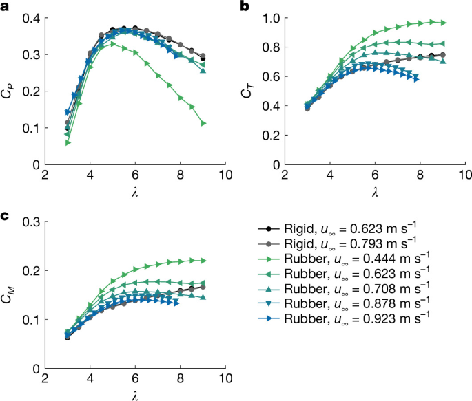
The principal measured quantities were torque (Q), thrust (T), flapwise root-bending moment (M) and angular velocity (ω). Measured loads and power are non-dimensionalized using standard turbine coefficients:
$${C}_{P}\equiv \frac{Q\omega }{\frac{1}{8}\rho {u}_{\infty }^{3}\pi {d}^{2}},$$
(3)
$${C}_{T}\equiv \frac{T}{\frac{1}{8}\rho {u}_{\infty }^{2}\pi {d}^{2}},$$
(4)
$${C}_{M}\equiv \frac{M}{\frac{1}{8}\rho {u}_{\infty }^{2}\pi {d}^{2}}.$$
(5)
The tip-speed ratio is defined as
$$\lambda \equiv \frac{\omega d}{2{u}_{\infty }},$$
(6)
where ω is the turbine angular velocity in radians per second.
Sensor accuracy and calibration uncertainties were propagated to the non-dimensional coefficients using standard bias-limit uncertainty analysis32, including thrust-torque transducer manufacturer specification (0.1% of full-scale capacity) and primary uncertainties in u∞, ω and geometric parameters. For the present setup, the maximum total bias limits is of order 10−2 for CP and of order 10−2 for CT (representative values). Supplementary Note 1 provides the full derivations and tables.
DIC and blade-shape reconstruction
Blade deformation was measured using phase-locked DIC with underwater cameras and LED illumination (LaVision). The camera system had a fixed focal length of 1.1 m and a field of view of approximately 0.87 m × 0.56 m, sufficient to capture the full blade span (0.56 m). Phase locking was achieved by using the proximity-sensor signal to trigger image acquisition as a blade passed a fixed azimuthal position, with a horizontal span and a downward tangential velocity. For each condition, between 89 and 447 instantaneous deformation fields were recorded over a 300 s period, depending on u∞ and λ.
Images were processed in LaVision DaVis 11 using a subset size of 21 × 21 pixels and a grid step size of 2 × 2 pixels, resulting in a spatial resolution of approximately 0.68 mm near the blade tip (approximately 2% of the tip chord). A reference image in quiescent water was acquired before each set of measurements. In the present configuration, DIC was used to measure the deformation of the suction-side surface of the blade. The full blade profile was reconstructed by combining the measured chord-line deformation with the known undeformed thickness distribution.
Fluid–structure interaction simulations
A bespoke fluid–structure interaction (FSI) solver was developed for the present study. The solver couples an in-house code based on blade element momentum theory (BEMT), with a panel method with an integral boundary-layer formulation (XFOIL), and a finite element analysis commercial software (Abaqus). The code uses a two-level iterative process, as schematically shown in Extended Data Fig. 9. The process begins with an initial blade geometry. In the outer loop, the BEMT solver is used to calculate the axial and tangential induction factors on a finite number of blade sections at different radial coordinates. Then, the flow velocity and angle of attack experienced by each blade section are computed. These values are used as initial conditions for the inner FSI loop. First, the pressure distributions around each blade section are computed with XFOIL. Then, the pressure distributions from each blade section are combined to obtain a three-dimensional pressure distribution on the blade, which is used as input to Abaqus, in which a new deformed shape is computed. The Abaqus model includes the steel spar. This new shape is then discretized into sections and returned to XFOIL to recalculate the pressure field. This iterative process continues until the blade shape converges. This deformed blade geometry at equilibrium is then fed back into the outer BEMT loop to update the induction factors. This entire two-level process is repeated until convergence. The power and thrust coefficients of the whole turbine are then computed by integrating the loads computed with XFOIL for each blade section and multiplying by three to account for the three-bladed turbine.
This code was used to design the stress-free mould shape for each blade stiffness, ensuring that the equilibrium blade shape matches the reference rigid blade at the design flow speed and tip-speed ratio. The model-scale simulations in Extended Data Figs. 4 and 5 are initialized with the mould geometry and use the actual stiffness of the metal spar and of the rubber. In the full-scale simulations (Extended Data Fig. 5), the stiffness of both the spar and the rubber is 10.6 times higher than at model scale to ensure that the model and full-scale Cauchy number for both the spar and the rubber is the same, where
$$\mathrm{Ca}\equiv \frac{\rho {u}_{\infty }^{2}}{E},$$
(7)
where ρ is the fluid mass density and E is the Young’s modulus.
{For more tech updates, stay tuned to our blog.|Keep following us for the latest insights.|Check back often for more exciting news!}