Experimental set-up

The set-up consists of the spatial DOP modulator interfaced separately with the high-dimensional PNN and the encryption–decryption system. These two blocks make a different use of scattering media and digital neural networks and are described hereafter in dedicated subsections.

Thank you for reading this post, don't forget to subscribe!

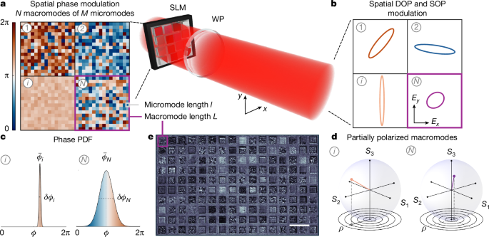
The DOP modulator is composed of a phase-only liquid-crystal-on-silicon SLM (Hamamatsu X13138, 1,280 × 1,024 pixels, 12.5 μm pixel pitch, 60 Hz frame rate) sandwiched between an input half-waveplate (HWP) and an output pair composed of a quarter-waveplate (QWP) and a HWP. An expanded beam from a continuous-wave laser (λ = 532 nm, 250 mW), with diagonal (D) polarization set by the input HWP, illuminates the SLM. The output QWP and HWP are mounted on high-speed motorized rotation stages and oriented at angles α and β, which are programmed together with the SLM. The WPs convert the phase delay ϕ imparted by a SLM pixel into a SOP set by (ϕ, α, β), as detailed in Supplementary Note 1. The DOP and SOP of a macromode are controlled through the four parameters (δϕ, \(\bar\), α, β). In the two-SLM implementation (Supplementary Fig. 4), two identical SLMs (Hamamatsu X15213-16L, 1,280 × 1,024 pixels, 12.5 μm pixel pitch, 60 Hz frame rate) are cascaded pixel-to-pixel by means of a 4f lens system with an inserted HWP at a fixed angle γ = 22.5°. The modulator is calibrated using polarimetry measurements performed by a rotating-WP polarimeter (Thorlabs PAX1000VIS, 0.25° accuracy) that measures S₁, S₂, S₃ and ρ.

Spatial modulation of the DOP and SOP is realized in two different configurations. In the first, the modulated beam is observed in a far-field plane located at a distance z from the SLM, whereas in the second, it is observed in the Fourier plane. We detail here the first configuration, as the experimental set-up is more versatile and does not require further optical components, and the Fourier implementation by means of a microlens array is detailed in Supplementary Note 6. The working distance z is set according to the micromode size l, which determines the diffraction length after which micromodes mix by propagation. At full resolution (N = 32 × 32), z is set to approximately 5 cm. For this z, the size of the macromode formed in the far field is comparable with its size L on the SLM.

The modulator is validated by a non-full-Stokes polarization camera (method 1) and a full-Stokes imaging system (method 2). The polarization camera (Thorlabs Kiralux, 2,448 × 2,048 pixels) acquires images (Fig. 3) of the linear polarization degree \(\nu =\sqrt{For more tech updates, stay tuned to our blog._^Check back often for more exciting news!+_Keep following us for the latest insights.^}/Keep following us for the latest insights._{0}\), azimuth θ = arctan(S₂/S₁)/2 and intensity S₀(x, y). Full-Stokes and DOP imaging is performed by carrying out Stokes measurements with the camera in intensity mode, that is, sequentially acquiring intensity projections of the beam profile through a QWP and a polarizer at different orientations⁵⁴. The accuracy of the spatial DOP and SOP modulation is evaluated by the \({\rm{RMSE}}=\frac{1}{N}{\sum }_{i}^{N}\sqrt{{\sum }_{k}|{S}_{k}^{{\rm{m}}}-{S}_{k}^{{\rm{p}}}{|}^{2}/3}\), in which superscripts ‘m’ and ‘p’ denote measured and programmed values, respectively.

Programming the spatial DOP modulator

The SLM active area is divided into N square macromodes (blocks of pixels). A macromode is further divided into M square micromodes, each consisting of l × l pixels, with l properly set to fill the SLM active area for a target resolution N. For instance, we use l = 12 pixels for M = 256 and N = 25 (Fig. 3d), that is, the micromode size is 150 μm in this case. The minimum macromode size required for accurate spatial modulation of the DOP and SOP is L = 25 pixels, achieved by using M = 25 micromodes of length l = 5 pixels (Fig. 3h). For high-resolution modulation (Fig. 3i), a few blank pixels of constant polarization are used to separate the macromodes and avoid their overlap owing to diffraction. The phase mask is constructed by assigning to all the pixels of the jth micromode a constant phase ϕ_j in the interval [0, 2π]. The value ϕ_j is randomly extracted from a Gaussian PDF that characterizes the ith macromode, \({{\mathcal{N}}}^{(i)}(\phi )=(1/\sqrt{2{\rm{\pi }}\delta {\phi }_{i}^{2}})\exp [-{(\phi -{\bar{\phi }}_{i})}^{2}/2\delta {\phi }_{i}^{2}],\) with standard deviation δϕ_i in [0, π/2] and mean \({\bar{\phi }}_{i}\) in [0, 2π]. By varying \(\bar{\phi }\), the SOP spans a trajectory on the Poincaré sphere that is tunable by the WP angles.

We calibrate the modulator by performing the analysis in Fig. 2 at different values of (δϕ, \(\bar{\phi }\), α, β). In Fig. 2, each data point corresponds to a single-mask experiment. Note that, as ρ tends to zero, the polarized component becomes less definite and, consistently, the measurement error on the Stokes parameters is larger. Averaging over several statistically equivalent masks allows us to reduce the noise observed in single-mask experiments (Supplementary Fig. 2). The DOP is calibrated using the average modulation and the fitting function ρ = aexp(−bδϕ²) + c. The measured SOP (Fig. 2b) is in close agreement with the polarization matrix model (Supplementary Note 2). We then construct a mapping between (S₁, S₂, S₃, ρ) and the four parameters (δϕ, \(\bar{\phi }\), α, β) = X. A target beam, spatially modulated in DOP and SOP, is generated by setting the vectors X⁽ⁱ⁾ accordingly. We study the dependence on the number of micromodes M in Supplementary Fig. 3. In the two-SLM implementation, the WP angles α and β are replaced by a second tunable phase \({\phi }_{2}^{(i)}\), which is set independently for each macromode and remains constant within it. In this case, the modulator is programmed by the vectors \({X}^{(i)}=(\delta \phi ,\bar{\phi },{\phi }_{2})\). The calibration of the two-SLM modulator is reported in Supplementary Fig. 5. The modulator is programmed using custom MATLAB codes.

Avoiding macromode crosstalk

To control the spatial modulation of the DOP and SOP, it is crucial that macromodes do not interact with each other. Any macromode crosstalk would degrade the modulation accuracy, as the state programmed on a macromode would affect its neighbours. To avoid macromode crosstalk, the far-field distance z must be chosen appropriately. As the interaction between two close micromodes and two close macromodes occurs at a distance on the order of their diffraction lengths z_l = πl²/λ and z_L = πL²/λ, respectively, the working distance must satisfy z_l ≪ z ≪ z_L. This condition is achieved easily for large macromodes (l ≪ L). For instance, L = 2.4 mm and l = 150 μm, as in Fig. 3d–f, yield approximately 0.1 m < z < 10 m. In this case, macromode crosstalk has a negligible effect. It becomes relevant when L and l are closer in value, as occurs when reducing M to maximize the number of addressable macromodes. In this case, crosstalk is avoided by using a few blank pixels that spatially separate adjacent macromodes. The length of this buffer area is chosen so that micromodes at the edge of two adjacent macromodes have no spatial overlap on propagation. The residual crosstalk is experimentally quantified in Supplementary Note 9. In Fig. 3i, in which l = 60 μm and z = 5 cm, we use d = 6 blank pixels. In the Fourier-plane implementation, macromode crosstalk is avoided by design because each microlens operates on a single macromode. This configuration is preferable for applications that require focused DOP-modulated light.

Encoding colours in polarization

To encode genuine RGB colours in polarization, SOP modulation alone is not sufficient. In fact, although we could associate some colours to different SOPs, such a mapping to the sphere surface does not preserve the essential property that gives any colour as a linear combination of the primaries. To overcome this limitation, DOP modulation is necessary. We use the map illustrated in Fig. 4a, given by \({S}_{1}=(2{\rm{R}}-1)/\sqrt{3}\), \({S}_{2}=(2{\rm{G}}-1)/\sqrt{3}\) and \({S}_{3}=(2{\rm{B}}-1)/\sqrt{3}\), with R, G, B ∈ [0, 1]. Note that many other maps are possible, including transformations that use a nonlinear relation or the spherical coordinates [θ, χ, ρ] on the Poincaré sphere. We can encode RGB colours with a precision of up to 8 bits per channel, determined by the SLM bit depth.

High-dimensional PNN

The optical part of the PNN is composed of n optical random layers formed by a stack of n diffusers (Thorlabs N-BK7 Ground Glass Diffusers with 120-, 200-, 600- or 1,500-grit polishes) and an optoelectronic layer implemented by a complementary metal–oxide–semiconductor (CMOS) camera (Basler a2A1920-160umPRO, 1,920 × 1,200 pixels, 12-bit pixel depth) positioned 10 cm away from the stack of diffusers. A 4 × 4-pixel binning is performed directly on the CMOS sensor, which implements an average pooling layer directly in hardware. The 300 × 300 acquired intensity values (12-bit precision) form the input to a digital backend. The digital network is a few-node network made of two fully connected layers with 40 hidden nodes and ten output nodes (output classes). The class is assigned by the softmax operation on the output vector and training is performed by using the Adam optimizer.

We classify colour images from the CIFAR-10 dataset⁵³, which consists of 60,000 32 × 32 RGB images of ten object classes with 6,000 images per class. These are divided into 50,000 training samples and 10,000 test samples. For comparison, we also classify the corresponding greyscale images obtained by converting the original RGB dataset. Images are polarization-encoded into N = 32 × 32 macromodes of size L = 25 pixels (Fig. 4c). The RGB to Stokes mapping in Fig. 4a is used. This performs a nonlinear operation on the input data. Note that phase encoding is also nonlinear⁵⁵. Therefore, the input nonlinearity has a minor role in the observed performance enhancement. Classification accuracy is averaged over repeated training and testing runs.

We model the high-dimensional PNN in terms of cascaded VTMs and partially coherent propagation⁵⁶, as detailed in Supplementary Note 7.

Scalability

As a high-dimensional encoder, the spatial DOP modulator supports a resolution that scales linearly with the number of SLM pixels, N = ξ⁻¹n_px, with ξ = L² = M × l² a set-up-dependent constant factor (Supplementary Table 1 reports a comparison of spatial optical encoders in PNNs). In our implementation with 32 × 32 macromodes, ξ ≈ 6 × 10² (Fig. 3h). According to this value, more than 10,000 macromodes can be generated with ultrahigh-definition SLMs (4K, n_px = 4,160 × 2,464). Therefore, a large-scale implementation is readily achievable with off-the-shelf components.

Multidimensional optical encryption system

Speckle-based encryption of polarization-encoded RGB images is performed using a 120-grit ground-glass diffuser as a scattering medium positioned in the focal plane of a lens (250 mm focal length), with the transmitted speckle pattern (ciphertext) collected by the CMOS camera. The speckle intensity is directly related to the input SOPs through the transmission tensor⁵⁷ of the diffuser. The acquired intensity images (1,200 × 1,200 pixels, 4,096 intensity levels) are downsampled to form a vector of size 1 × 90,000. The DNN consists of two fully connected layers, with w × N hidden nodes and 3 × N output nodes, connected by means of batch normalization and ReLU activation. The hyperparameter w sets the hidden-layer size and is tuned to optimize the decryption accuracy (w = 4 for the results in Fig. 5). The 3 × N output vector contains the values S₁, S₂ and S₃ of the N macromodes. The decrypted image is obtained by inverse mapping to the RGB values with the chosen relation [R, G, B] ↔ [S₁, S₂, S₃]. The error owing to an incorrect map (security key) is shown in Supplementary Fig. 17.

The decryption DNN used in Fig. 5 has nearly 3.8 × 10⁸ learnable parameters (12.2 Gbit at 32-bit precision). It is trained on a dataset of 20,000 plaintext–ciphertext pairs. The fidelity of the decrypted image is quantified by the PCC, an easily interpretable metric. We can encrypt any RGB image up to 32 × 32 pixels. In Fig. 5, we encrypt CIFAR-10 images to demonstrate operation at the maximum supported resolution.