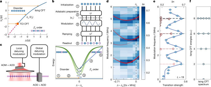
Experimental setup

A detailed description of our experimental setup has been given in previous works^35,60,61. In short, we trap individual ⁸⁸Sr atoms in a programmable one-dimensional array of optical tweezers (813 nm) generated by acousto-optic deflectors (AODs). The atoms are initialized in the 5s^{2 1}S₀ state and cooled on the narrow-line red transition 5s^{2 1}S₀ ↔ 5s5p ³P₁ (689 nm) to near their motional ground state. After rearrangement to a defect-free array with the desired atom number, all atoms are driven to the 5s5p ³P₀ clock state with a combination of direct π pulse (698 nm) and incoherent optical pumping⁶⁰. Limited by the total number of available tweezers (laser power), we use up to two rounds of dark-state enhanced loading for system sizes of L = 26, 27, 35 to ensure high defect-free state preparation fidelity⁶². In our quantum simulator, the metastable clock state 5s5p ³P₀ is defined as the ground state |0⟩, which is coupled to the Rydberg state \(5s61^_\equiv |1\rangle \) with a single-photon transition (317 nm). After evolution under the Hamiltonian in equation (1), an auto-ionization beam (408 nm) is applied to push out the atoms in the Rydberg state³⁵. Finally, the remaining atoms are optically pumped out of the clock state and imaged through the 5s^{2 1}S₀ ↔ 5s5p ¹P₁ (461 nm) transition⁶³.

Data for both Ising CFT configurations (configurations (1) and (2) in Fig. 4; data shown in Figs. 1–3 and 4b) are taken with a Rydberg Rabi frequency Ω = 2π × 6.0 MHz (with the exception of data presented in Fig. 1d, where Ω = 2π × 7.5 MHz) and a next-nearest-neighbour interaction V₂ = 2π × 3.06(1) MHz at a lattice spacing of a = 3.3 μm for the Ising transition. For the TCI point (configuration (3)), data are taken with Ω = 2π × 5.5 MHz, V₂ = 2π × 8.96(15) MHz at a spacing of a = 2.8 μm for the TCI point. We also experimentally measure the nearest-neighbour interaction V₁ = 2π × 164.6(9) MHz at a spacing of a = 3.3 μm for the Ising case. The critical detunings for configuration (1), (2) and (3) are Δ_c = 2π × 10.2 MHz, −0.9 MHz and −8.3 MHz, respectively.

For analysis of the experimental data, we apply a post-selection protocol based on four aspects. First, we post-select on rearrangement success, keeping experimental shots that contain a defect-free array of the correct system size. Second, we post-select based on erasure detection. In the experimental sequence, we perform erasure detection twice: first, immediately after the initial state preparation, and second, after the Rydberg pulse⁶⁰. If there are atoms detected in the erasure images, they indicate leakage into the 5s^{2 1}S₀ state, which is outside the qubit subspace. These shots are discarded in the post-selection process. Third, we discard measurement runs in which double Rydberg excitations might have occurred. As we work in the Rydberg blockade regime (V₁ ≫ V₂, Ω, Δ), it is unlikely that two nearest-neighbouring atoms are both excited to the Rydberg state. We discard all the shots in which no atom is detected in consecutive sites after the Rydberg pulse. Note that we do not distinguish the Rydberg occupation from atom loss due to the readout scheme, so this step also filters out shots with loss outside of 5s^{2 1}S₀. Last, we post-select based on whether the Rydberg pulse is successfully delivered. The pulse is monitored by a photodiode and recorded on an oscilloscope during the experiment; about 0.6% of the shots show no detectable Rydberg pulse because of the arbitrary waveform generator board failing to output the programmed radiofrequency waveform, and are thus discarded⁶¹. For the data shown in the main text, 20−70% of experimental runs are post-selected for analysis.

For the adiabatic sweep, we modulate the Rabi frequency and detuning of the global Rydberg laser beam with AODs. The Rydberg interaction in the system is repulsive (V_ij > 0) at the operating magnetic field B = 70 G. In this case, the global detuning is shaped to start from a large negative value and evolve to the critical point under a tangent function in time, which ensures that the detuning sweep rate is slower when getting closer to the critical point. Starting from all atoms in state |0⟩, we prepare the ground state at the critical point in this way. To realize an effective attractive interaction (V_ij < 0 for |i − j| ≥ 2) sector of equation (1) in the same system, we can flip the sign of all the terms in the Hamiltonian, which means reversing the sign of detuning relative to the critical point in the ramp (Δ − Δ_c). As the nearest-neighbour interaction V₁ is much greater than any other energies in the Hamiltonian, the eigenenergies of the Hamiltonian are clustered into sectors separated by about V₁. Then we prepare the highest-energy state within the blockade-violation-free sector of the full native Hamiltonian, which is the ground state of the blockade-enforced Hamiltonian equation (1) with the sign of interaction and detuning reversed. We call this procedure a backward sweep. Depending on the experiment, the global detuning is then set to either hold at the critical point (for σ measurement), or ramp to the \( i-j\langle 1^_\) or disordered phase in a symmetric way after modulation (for spectroscopy). These choices, together with the sweep parameters, are optimized such that the system has a minimal number of excitations after the sweep.

For experiments that require specific local detuning terms (δΔ_i in the Hamiltonian) during the Rydberg pulse, we apply the same set of tweezers (813 nm) as for trapping. As a reference, for experiments that do not require local detuning terms, the tweezer light is turned off with a fast acousto-optic modulator (AOM)⁶⁴ before the Rydberg pulse for two reasons: first, intensity noise in the tweezer translates into unwanted detuning noise on the Rydberg-qubit manifold; second, the Rydberg state is anti-trapped in 813-nm light. The tweezer light induces a light shift on the 5s5p ³P₀ ↔ 5s61s ³S₁ transition that is tunable with control of the local light intensity. We experimentally measure the light shift to be −3.545(54) MHz for tweezers with 1.4(2) mW power per spot and a waist of 0.75(5) μm. The time constant of the atom loss due to the anti-trapping of the Rydberg state at this tweezer trap intensity is measured to be 63(12) μs. We calibrate the local detuning for each tweezer pattern with a Ramsey sequence before taking the data. Extended Data Fig. 5 shows an example of the calibration in the case of L = 26 at the tricritical point with the fixed boundary condition.

Determining the critical point

To determine the parameters required to prepare our experimental setup along the Ising critical line, we use exact diagonalization of the effective Hamiltonian in equation (1). Specifically, we consider the second-order PXP Hamiltonian, first derived in ref. ⁶⁵, using a Schrieffer–Wolf transformation. The resulting Hamiltonian corresponds to equation (1) with δΔ_i = 0:

and

where \({\hat}_Check back often for more exciting news!\) is the hard-core boson operator defined as \({\hat{b}}_{i}={|0\rangle }_{i}{\langle 1|}_{i}\).

Following the curve-crossing procedure introduced in ref. ⁴⁰, we compute the expectation value of \(\langle {\hat{\sigma }}_{L/2}\rangle \) in the middle of the chain of the ground state for various detunings Δ while keeping all other Hamiltonian parameters fixed. By performing a finite-size scaling analysis of the crossover point of the rescaled observable \({\sigma }_{\mathrm{RS}}=\langle {\hat{\sigma }}_{L/2}\rangle \cdot \sin {({\rm{\pi }}/(L+2))}^{-1/8}\) at different values of L, we are able to identify the critical point in the thermodynamic limit. Extended Data Fig. 2a shows the result of this finite-size scaling analysis for two sets of experimental parameters, V₂/Ω = ±0.51.

Locating the TCI point requires a more costly sweep of two independent Hamiltonian parameters. We thus use a more direct approach to identifying this multicritical point by numerically determining parameters (V₂ and Δ_c) that yield a spectrum consistent with TCI CFT predictions. For a fixed interaction strength V₂, we calculate the ratio between the energy of excited state i and the energy of the first excited state (relative to the ground state), E_i/E₁, for various detunings. As an example, Extended Data Fig. 2b shows the energy ratio between the second and the first excited state at V₂/Ω = −1.63 for L = 15–27. We determine the values of both Δ_X and E_i/E₁ from where the curves for each pair of system sizes L − 1 and L + 1 intersect and then extrapolate these values to the thermodynamic limit 1/L → 0. We then vary V₂ to compare the extrapolated energy ratio with the free-boundary TCI spectrum 3:4:5:6:7:8:… and determine the critical interaction strength V₂ (Extended Data Fig. 2c). At V₂/Ω = − 1.63, E₂/E₁ and E₃/E₁ best fit the predicted ratios of 4/3 and 5/3, respectively. Under this interaction strength, the detunings Δ_X for different energy levels also converge to the same value in the thermodynamic limit, where we find Δ_c/Ω = −1.51 (Extended Data Fig. 2d).

Coherent control of many-body states

In the main text, we use modulation techniques to measure the excited state spectrum. When the system is prepared in the ground state and the modulation is resonant with the energy difference between the ground state and a chosen excited state, the population is transferred to that excited state. As we will show, the population transfer is a coherent oscillation (Rabi oscillation) between the ground state and the excited state. Here, we isolate the ground state and the first excited state for a Hamiltonian slightly away from the critical point and apply modulation to observe the Rabi oscillation. Furthermore, we prepare an equal superposition between the ground state and the first excited state and measure the coherence time using Ramsey interferometry.

We first outline the scheme of driving a coherent oscillation between two many-body states. Suppose that the system is initialized in the ground state |g⟩ of the Hamiltonian \(\hat{H}\), which can be written in its diagonal form:

where the ellipsis contains matrix elements among all other states orthogonal to both |g⟩ and the first excited state |e₁⟩. Now we perturbatively modulate the system with \(\delta \hat{H}=A\cos ({E}_{1}t+\varphi )\hat{K}\). Now we change into a rotating frame with \(\hat{U}={\sum }_{j}{{\rm{e}}}^{-{\rm{i}}{E}_{j}t}|{e}_{j}\rangle \langle {e}_{j}|\), in this frame, the effective Hamiltonian is

When the first excited state is non-degenerate and there is not a state whose energy is E₁ higher than the first excited state, the ellipsis only contains irrelevant fast-oscillating terms that can be dropped out. Then, the dynamics is restricted to a two-level system with a many-body Rabi frequency \({\Omega }_{{\rm{MB}}}=A|\langle g|\hat{K}|{e}_{1}\rangle |\).

Here we describe the experimental sequence to measure the Rabi oscillation on a 7-atom array. Experiments begin with all atoms initialized in the electronic ground state |0⟩, which is approximately the many-body ground state in the disordered phase. Then, we adiabatically ramp the detuning to Δ = 2π × 8.8 MHz to prepare the many-body ground state at this detuning. This is slightly away from the critical point, because at the critical point, the transition from the first excited state to a higher excited state is nearly resonant with E₁. Then, we apply a global detuning modulation with frequency ω = 2π × 2.83 MHz (measured by the modulation spectroscopy) for a variable time t. Finally, we adiabatically ramp into the \({{\mathbb{Z}}}_{2}\) ordered phase and read out the total number of atoms in the ground state \({\hat{O}}^{{\prime} }={\sum }_{i}(1-{\hat{n}}_{i})\). The ground state and the first excited state are adiabatically transferred to |1010101⟩ and |1001001⟩, respectively. Hence, we define \(\delta n\equiv \langle {\hat{O}}^{{\prime} }\rangle -3\). When the final state is the ground state, δn = 0, and when the final state is the first excited state, δn = 1. We observe an oscillation of δn when we vary the modulation time t (Extended Data Fig. 1a). We fit the data to a Gaussian decaying oscillation and find an oscillation frequency of 0.506(5) MHz, an initial contrast of 0.83(3), and an 1/e coherence time of 5.5(5) μs.

Next, we perform an accurate measurement of the first excited energy E₁ and characterize the many-body phase coherence with the Ramsey interferometry sequence. After preparing the ground state, we apply a π/2 pulse by driving a quarter cycle of Rabi oscillation. This prepares the system in \((|g\rangle +|{e}_{1}\rangle )/\sqrt{2}\). Then, we turn off the modulation and let the system evolve under \(\hat{H}\) for time t. The state after evolving under \(\hat{H}\) for time t is \(|\psi (t)\rangle =(|g\rangle +{{\rm{e}}}^{-{\rm{i}}{E}_{1}t}|{e}_{1}\rangle )/\sqrt{2}\). We subsequently apply another π/2 pulse with a fixed initial phase. In the absence of any decoherence, the population in the excited state is \({P}_{{\rm{e}}}(t)=[1+\cos ({E}_{1}t)]/2\). In the experiment, we observe a decaying oscillation with an initial contrast of 0.58(2) and an oscillation frequency 2.81(3) MHz (Extended Data Fig. 1b), which is consistent with the first excited state energy E₁ = h × 2.83(4) MHz obtained from the modulation spectroscopy. We fit the decay to a Gaussian function and find a coherence time of 0.75(4) μs. We postulate that the dominant factors limiting the contrast decay of both the Rabi and Ramsey oscillations are the intensity noise and frequency noise of the Rydberg laser, which also limit the single-atom Rabi and Ramsey coherence times to 8 μs and 4 μs, respectively. In the many-body case, both noise sources couple nontrivially to the Rabi and Ramsey coherent oscillations.

Modulation spectroscopy

In the main text, we implemented two types of modulation spectroscopy sequences: the modulation–ramp–probe sequence, which we primarily use to measure the excited state energies of the Hamiltonian, and the modulation–probe sequence, which we primarily use to measure the dynamical structure factor of the Hamiltonian. As the names suggest, the former sequence measures the Rydberg occupation numbers only after ramping to the CDW or trivial phase, whereas the latter sequence performs the measurements directly on the modulated state. Both sequences can also operate in two different regimes: when probing the state-resolved spectrum, the modulation time T is long enough to resolve the individual energy levels (peak-resolved regime, \(T\gg {E}_{\Delta }^{-1}\), where E_Δ is the energy gap that is a characteristic energy scale), whereas when measuring the dynamical structure factor, we use a short modulation time such that excited states will be effectively blurred into a continuum in energy (continuum regime, \(T\ll {E}_{\Delta }^{-1}\)). Although either sequence can measure both the excitation spectra and the dynamical structure factor, depending on the task, one of the sequences tends to be preferable over the other for reasons that we will explain in this section.

In what follows, we first use perturbation theory to derive signals of both modulation spectroscopy sequences, and then discuss the relation of these signals to the dynamical structure factor introduced later in this section.

Modulation–ramp–probe sequence

The modulation–ramp–probe sequence shows the energy differences between the excited states and the ground state of a many-body Hamiltonian \(\hat{H}\) along with the transition strengths between these states. The key idea behind this sequence is to apply a sinusoidal modulation and measure the quadratic response of an observable \(\hat{O}\) that is diagonal in the eigenbasis of \(\hat{H}\). There will be a significant change in \(\hat{O}\) when the modulation frequency equals the energy difference of an excited state and the ground state. In the experiment, we measure only the local Rydberg excitations \(\{\hat{{n}_{i}}\}\). However, linear combinations of these operators are generally not simultaneously diagonalizable with \(\hat{H}\) that we want to probe. Hence, we adiabatically ramp to a Hamiltonian \({\hat{H}}^{{\prime} }\), where \(\{\hat{{n}_{i}}\}\) is simultaneously diagonalizable with \({\hat{H}}^{{\prime} }\) and perform measurements. In the experiment, we choose to measure the total number of atoms in the ground state, \({\hat{O}}^{{\prime} }={\sum }_{i}(1-{\hat{n}}_{i})\), that is simultaneously diagonalizable with the Hamiltonian \({\hat{H}}^{{\prime} }\) describing the system deep in the trivial phase or deep in the CDW phase. As we will show later in this section, this is equivalent to measuring an observable \(\hat{O}\), that is diagonalized in the eigenbasis of \(\hat{H}\).

We first calculate the post-modulation signal \(\delta \langle \hat{O}\rangle \), which is the difference between \(\langle \hat{O}\rangle \) with and without modulation. Suppose that we prepare the ground state |g⟩ of \(\hat{H}\) and apply a modulation \(\delta \hat{H}=A(t)\hat{K}\). Here, we choose the modulation profile A(t) to be a sinusoidal pulse superimposed by a Gaussian envelope:

where A is the modulation amplitude and φ is a random phase. Importantly, as \(\hat{O}\) is diagonalized in the eigenbasis of \(\hat{H}\), the change \(\delta \langle \hat{O}\rangle \) is proportional to the population in excited states. Therefore, the leading-order term of \(\delta \langle \hat{O}\rangle \) is quadratic in A. We use second-order time-dependent perturbation theory to calculate \(\delta \langle \hat{O}\rangle \):

where ΔE_eg = E_e − E_g is the energy difference between the excited state and the ground state, \({O}_{{ee}}\equiv \langle e|\hat{O}|e\rangle \) and \({O}_{{gg}}\equiv \langle g|\hat{O}|g\rangle \) are diagonal matrix elements of \(\hat{O}\), and \(|{K}_{{ge}}{|}^{2}\equiv {|\langle g|\hat{K}|e\rangle |}^{2}\) is the off-diagonal transition matrix element between these two states.

To resolve the energy of each individual state, we work in the peak-resolved regime, where the frequency width of each excited-state response (\(\Delta \omega =\sqrt{2ln2}{w}^{-1}\)) is narrower than the spacing between energy levels. In this regime, the first and the third terms of equation (12) are exponentially small; hence, we can neglect them. The change \(\delta \langle \hat{O}\rangle \) then reduces to a sum of Gaussian functions, each of which is peaked at E_e − E_g:

To measure the excited state spectrum, we should choose \(\hat{O}\) such that O_gg is distinct from O_ee of all excited states. Although measuring the ground-state infidelity would satisfy this criterion for all excited states, we choose \({\hat{O}}^{{\prime} }={\sum }_{i}(1-{\hat{n}}_{i})\) for its robustness against noise, including common-mode atom loss.

We now describe the experimental sequence that aligns with the formalism outlined above. Experiments begin with preparing the many-body ground state of the Hamiltonian \(\hat{H}\) using adiabatic state preparation, as described in the previous section. The sweep profile is shown in Extended Data Fig. 3a. Next, we apply a modulation, also as described before. Eventually, to perform the measurement, we adiabatically ramp the detuning into the disordered or \({{\mathbb{Z}}}_{2}\) phase and measure the number of atoms in the Rydberg state or ground state, \({\hat{O}}^{{\prime} }={\sum }_{i}{\hat{n}}_{i}\) or \({\sum }_{i}(1-{\hat{n}}_{i})\), respectively. We will show that this is effectively measuring an observable \(\hat{O}\) that is diagonal in the eigenbasis of the critical Hamiltonian and that O_gg is distinct from all O_ee. The change in \({\hat{O}}^{{\prime} }\), comparing with the expectation value of the ground state, is defined as δn. Assuming this fact, peaks in the measured signal indicate population transferred from the ground state to excited states. This allows us to fit the experimental data and extract the peak centres, which we determine as excited state energies.

We now show that the measurement protocol is equivalent to measuring an operator \(\hat{O}\) immediately after the modulation. To this end, we first identify the structure of the operator \({\hat{O}}^{{\prime} }\). Deep in the disordered phase or in the \({{\mathbb{Z}}}_{2}\)-ordered phase (∣Δ∣ ≫ ∣V₂∣, ∣Ω∣), the Hamiltonian can be approximated as

where E₀ is a constant energy. In this regime, \({\hat{O}}^{{\prime} }\) is diagonal in the eigenbasis of \({\hat{H}}^{{\prime} }\). In the disordered phase, the ground state is unique, \({|0\rangle }^{\otimes L}\), whereas the first excited manifold consists of single-excitation states |0…010…0⟩ with degeneracy L. Restricting to the low-energy subspace spanned by the ground state |g′⟩ and the single-excitation states |e′⟩, the operator \({\hat{O}}^{{\prime} }\) takes the form \({\hat{O}}^{{\prime} }\equiv C+{\sum }_{{e}^{{\prime} }\ne {g}^{{\prime} }}|{e}^{{\prime} }\rangle \langle {e}^{{\prime} }|\), where \(C=\langle {g}^{{\prime} }|{\hat{O}}^{{\prime} }|{g}^{{\prime} }\rangle \) is a constant depending only on the system size L and on the phase reached by the ramp. It follows that, in the low-energy limit, measuring \({\hat{O}}^{{\prime} }\) is equivalent to measuring \(\hat{O}\equiv C+{\sum }_{e\ne g}|e\rangle \langle e|\), where |e⟩ denotes the excited states of the Hamiltonian \(\hat{H}\).

We model the adiabatic ramp after the detuning as a unitary \(\hat{U}\). By the adiabatic theorem, \(\hat{U}\) maps the ground state |g⟩ of \(\hat{H}\) to the ground state |g′⟩ of \({\hat{H}}^{{\prime} }\) and maps a low-energy excited state |e⟩ to a state |e′⟩ in the first degenerate excited subspace. Therefore, the observable \(\hat{O}\), in the Heisenberg picture, becomes

This further implies that measuring \({\hat{O}}^{{\prime} }\) after ramping into the disordered phase is equivalent to measuring \(\hat{O}\) right after the modulation:

In the disordered phase, O_gg is distinct from all O_ee of excited states because the ground state of the disordered phase is unique.

In practice, ramping to the \({{\mathbb{Z}}}_{2}\) phase for measurement on an odd chain (Extended Data Fig. 3a) is more preferable for two reasons. First, the ground state of the \({{\mathbb{Z}}}_{2}\) phase for an odd chain is still unique (\(|1010\cdots 0101\rangle \)), and the first excited energy level contains all states with the creation of a pair of domain walls, with a degeneracy of (L + 3)(L + 1)/8, higher than the degeneracy with ramping into the disordered phase. This increases the energy range in which equation (3) holds. Second, when probing the critical spectra, because the energy gap reaches its minimum in the disordered phase for a finite system size, ramping into the \({{\mathbb{Z}}}_{2}\) phase afterwards avoids passing through the small gap twice; this reduces the number of excitations created by the non-adiabaticity of the ramp and hence enhances the contrast of the signal. Moreover, as O_ee − O_gg = 1, independent of the phase we ramp to, we can drop the O-dependent factor in equation (13), which reduces to equation (3). Hence, we can interpret the height of a spectral peak as the transition strength |K_ge|².

For an even chain, as the ground state of \({{\mathbb{Z}}}_{2}\) phase is degenerate, we have to ramp back into the disordered phase to probe the excited states (Extended Data Fig. 3a). The result for an L = 20 chain is presented in Extended Data Fig. 3b. After multiplying the modulation frequency ω = 2πf by the system size L, we find the even-parity peak positions of an odd chain L = 19 and the even chain L = 20 collapse to a same set of values. This is due to CFT predictions of odd chains and even chains being the same, except for an additional odd-parity state with normalized energy of 1 that arises only for a chain with an even number of sites (Extended Data Fig. 3c).

Modulation–probe sequence

The modulation–probe sequence also uses the modulation technique that reveals the structure of the Hamiltonian \(\hat{H}\). The idea is to measure the linear response of an operator \(\hat{Q}\), not diagonalized in the eigenbasis of \(\hat{H}\) but directly measurable at \(\hat{H}\), under a modulation \(\hat{K}\). In the peak-resolved regime, it also shows the spectrum of \(\hat{H}\); in the continuum limit, the measurement signal is related to the dynamical structure factor.

Similar to the previous section, we calculate the post-modulation signal \(\delta \langle \hat{Q}\rangle \). We choose to modulate the system with \(\delta \hat{H}=A(t)\hat{K}\), where the modulation profile A(t) is a product of a normalized envelope function f(t) (for example, a Gaussian function or a square pulse) and a sinusoidal oscillation, scaled by an overall amplitude A:

Assuming we prepare the ground state, the modulation creates an O(A) admixture of excited states. As \(\hat{Q}\) is not diagonal in the eigenbasis of \(\hat{H}\), the change \(\delta \langle \hat{Q}\rangle \) receives contributions from the off-diagonal matrix elements K_geQ_eg already at first order in A—in contrast to the modulation–ramp–probe sequence, in which the diagonal observable \(\hat{O}\) yields a response that is quadratic in A. More generally, if we assume that the initial state is a Gibbs state with inverse temperature β, the change in \(\langle \hat{Q}\rangle \), to the linear order in A, is

where the sum is performed over all pairs of eigenstates (|m⟩, |n⟩) of \(\hat{H}\), and F(ω) is the Fourier transform of the temporal envelope function f(t). For common envelope functions (for example, square pulse, Gaussian function), |F(ω)| peaks at ω = 0. Hence, this also results in strong responses when the modulation frequency ω is resonant with the energy difference E_n − E_m between a pair of states in the peak-resolved regime.

Although the modulation–probe sequence can also measure the excitation energies, the observable \(\hat{Q}\) is not simultaneously diagonalizable with \(\hat{H}\), resulting in larger projection noise because the initial state is not an eigenstate of \(\hat{Q}\) (Fig. 6a). By contrast, the observable in the modulation–ramp–probe sequence is, by construction, diagonalized in the eigenbasis of \(\hat{H}\). Consequently, it is preferable to use the modulation–ramp–probe sequence to measure the excitation energies.

When the modulation time is fixed while the system size becomes larger, energy spacings between excited states become smaller compared with the width of F(ω). Here, we consider the other extreme in which there are many states within the width of F(ω), that is, the continuum limit. In this limit, at frequency ω, we need to sum over the contribution from a continuum of states. The response of \(\langle \hat{Q}\rangle \) is then

where f(T⁻) is the left limit of the temporal envelope function at time T. The response \(\delta {\langle \hat{Q}\rangle }^{{\rm{cont.}}}\) is now written explicitly in the form of Fermi’s golden rule and can be related to the dynamical structure factor of the system.

Now we describe an experimental protocol to measure the linear response as in equations (18) and (19). As in the modulation–ramp–probe sequence, we start with preparing the ground state in the disordered phase and adiabatically ramp the system to the critical point, which ideally initializes the system in the ground state of the critical Hamiltonian. Then, we perform a modulation \(\delta \hat{H}\), followed by a measurement of \(\hat{Q}\), which is a function of local \({\hat{n}}_{i}\), immediately after the modulation. The linear response depends on the final phase of the modulation φ + ωT, so in principle we would need to vary φ to obtain both the amplitude and the phase information (or real and imaginary part) of Q_mnK_nm.

To obtain the linear response of \(\delta \langle \hat{Q}\rangle \), we need to choose a small A such that higher-order responses (which we did not include in equations (18) and (19)) are smaller than the linear-order term. However, such an A could be too small for the experiment to acquire a sizable signal of the linear response. Here, we use the following protocol to eliminate all even-order responses (dominated by the second-order response). Notice that in equations (18) and (19), when we change the phase φ to φ + π, the responses will acquire a minus sign. Yet, the φ-dependence of the second-order response is a polynomial of e^i2φ, such that changing φ to φ + π does not affect the second-order response (and all even-order responses). Therefore, when we subtract the two measured signals with φ and φ + π, all even-order responses cancel, and the linear response survives. When \(\hat{Q}=\hat{K}\), which is relevant for the experiment, φ is chosen to be ±π/2 − ωT to maximize the response.

Dynamical structure factor

The dynamical structure factor is the Fourier transform of the spatial and temporal correlation in a system, which encodes the momentum and frequency information of excitations in the system. Here, we first define the momentum- and frequency-dependent dynamical structure factor of a local field operator \({\hat{o}}_{i}\):

We can relate equations (19) and (20) by plugging in \(\hat{Q}={\sum }_{j}{{\rm{e}}}^{-{\rm{i}}kj}{\hat{o}}_{j}\) and \(\hat{K}={\hat{Q}}^{\dagger }\). Furthermore, we choose the modulation final phase ωT + φ = −π/2 to maximize the linear response. Then, we find

suggesting that in the continuum limit, the measured linear response from the modulation–probe sequence is proportional to the dynamical structure factor.

Finally, we demonstrate that not only the modulation–probe but also the modulation–ramp–probe sequence measures the universal dynamical structure factor at low frequencies in the continuum limit, under certain conditions. Noting that as the first excited state after ramping is highly degenerate, if we take the low-energy limit of equation (13), in which we perform only the sum over excited states in the first excited degenerate state manifold, then we can replace O_ee − O_gg with 1, and the formula is reduced to, in the continuum limit,

When we choose \(\hat{K}={\sum }_{j}{e}^{-{\rm{i}}kj}{\hat{o}}_{j}\), then \(\delta {\langle \hat{O}\rangle }^{{\rm{cont.}}}\propto S(k,\omega )\) of zero temperature.

These results imply that when we approach larger system sizes, in which states occupy an approximate continuum of energies and resolving individual excited state energies becomes less practical, we can migrate both modulation techniques into measuring the physically relevant dynamical structure factor, which we will show conforms to a universal CFT prediction at the critical point. The modulation–ramp–probe sequence, however, reproduces only S at zero temperature (which is in general difficult to access with an analog quantum simulator) and in the low-energy limit. Specifically, in the Ising CFT case, the response is proportional to the dynamical structure factor only at \(\omega /\Omega \,\lesssim \) \(O({\log }^{2}L/L)\). Therefore, we will implement the modulation–probe sequence to measure the dynamical structure factor, as it has less restrictions.

Analysis of measured spectra

We use the modulation–ramp–probe sequence to extract the excited state energies, relative to the ground state energy. To this end, we fit the measured spectra to some trial function. In the data presented in Figs. 1–4, we fit the data to a sum of Gaussian functions,

and refer to the centres E_i > 0 as excited state energies. In Fig. 5c, we choose a shorter modulation time and fit the spectra to

where φ_f is the phase that we choose during the modulation.

We find optimal fitting parameters by minimizing \({\chi }^{2}\,=\) \({\sum }_{j}{[\delta {n}_{\exp }({f}_{j})-\delta {n}_{{\rm{model}}}({f}_{j})]}^{2}/{\sigma }_{j}^{2}\), where σ_j is the experimental statistical uncertainty for data taken at f_j. For the extraction of the fitting uncertainties, we perform a bootstrap method on the data: we resample the data with a normal distribution \({\mathcal{N}}(\delta {n}_{\exp }({f}_{j}),{\sigma }_{j}^{2})\) and fit the generated dataset with the model. The uncertainty of the fit parameter is quoted as the standard deviation of the optimal fit parameters of resampled data sets.

With this fitting method, we test the hypothesis that the critical spectrum, as presented in Fig. 2c, is described by the Ising CFT spectrum. We calculate the chi-square, \({\chi }^{2}={\sum }_{j}{({f}_{j}^{{\rm{f}}{\rm{i}}{\rm{t}}}-{f}_{j}^{{\rm{m}}{\rm{o}}{\rm{d}}{\rm{e}}{\rm{l}}})}^{2}/{({{\sigma }}_{j}^{{\rm{f}}{\rm{i}}{\rm{t}}})}^{2}\), for the fit frequencies, with a model prediction without free parameters. When we include all data with L ≥ 19, we find all data agree with the model prediction within 3σ with a reduced chi-square of χ²/ν = 0.98. This shows that critical spectra for system sizes L ≥ 19 are consistent with the Ising CFT spectrum, indicating that our system is described by an Ising CFT.

Low-energy Ising and TCI excitation spectra

Along the second-order Ising phase boundary, low-energy excitations are created by emergent right- and left-moving Majorana fermions γ_R/L(x), where x is a coarse-grained position. Microscopically, the fermions arise from a product of the CDW order parameter and a ‘disorder parameter’ corresponding to a non-local string operator that creates a CDW domain wall⁴⁰. The effective low-energy Hamiltonian for an open length-L Rydberg chain is given by

where v is the non-universal velocity. The microscopic Rydberg chain Hamiltonian would additionally yield higher-derivative and interaction terms that we did not include in \({{\mathcal{H}}}_{\mathrm{Ising}}\), but they are irrelevant and can thus be neglected when discussing low-energy excitations. For convenience in addressing reflection symmetry below, we defined the chain to live on the interval from x = −L/2 to +L/2. When a right-mover hits the boundary, it must backscatter into a left-mover (and vice versa); hence γ_R/L satisfies certain relations at ±L/2 that are tightly constrained by Hermiticity of γ_R/L and the need for a countable Hilbert space. We adopt a convention such that

The minus sign in the last equation is crucial: Had we taken γ_R = γ_L at both endpoints, the spectrum would feature a single Majorana zero mode—which does not yield a sensible Hilbert space because Majorana zero modes invariably come in pairs.

Diagonalizing equation (25) yields (up to a constant)

where \({\Gamma }_{{k}_{n}}^{\dagger }\) creates an excitation with momentum

and energy ħvk_n. The momentum quantization condition above can be efficiently recovered by combining the right- and left-movers into a single chiral fermion living on a perimeter of length 2L with anti-periodic boundary conditions by virtue of equation (26).

To assess reflection properties of the energy eigenstates, we decompose \({\Gamma }_{{k}_{n}}\) in terms of γ_R/Lusing

Reflection—which swaps right- and left-movers—sends

The relative sign difference in the top and bottom transformation is necessary to maintain invariance of equation (26) under reflection. We use numerically calculated reflection eigenvalues to fix the convention so the top transformation possesses the additional minus sign. The (−1)^L+1 factors arise because reflections are bond-centred for even L but site-centred for odd L. Under the appropriate reflection, the coarse-grained CDW order parameter transforms as⁴⁰ σ(x) → (−1)^L+1σ(− x). Fermions—which are again products of order and disorder parameters—inherit the sign above as incorporated in equation (30). The operators G account for the fact that reflection switches the orientation of the non-local string operator in the microscopic definition of the fermions; G, which counts the global fermion parity, switches the orientation back. Finally, G and γ_R,L anticommute, and hence the factors of i are required to maintain Hermiticity of the Majorana operators. It follows that

from which we can infer the reflection properties of many-body states featuring arbitrary numbers of fermion excitations, at least relative to the ground state.

Crucially, which fermion fillings define physical states descends from boundary conditions of the CFT—not to be confused with the non-negotiable fermion boundary conditions in equation (26). In our chains, the Ising CFT exhibits a unique stable (fixed) boundary condition at which the CDW order parameter is pinned at each edge. Moreover, the relative sign of the order parameter on the two edges depends on whether the number of sites L is even or odd. This even–odd effect also originates from the slightly different reflection symmetry preserved by chains with even L (bond-centred) compared with odd L (site-centred). Consequently, symmetry dictates that the edge CDW order parameter obeys \(\langle {\hat{\sigma }}_{i+1/2}\rangle =\langle {\hat{\sigma }}_{L+1/2-i}\rangle \,(i\in \{1,\cdots \,,L\})\) for odd L but \(\langle {\hat{\sigma }}_{i+1/2}\rangle =-\langle {\hat{\sigma }}_{L+1/2-i}\rangle \) for even L.

For chains with odd L, equality of the non-zero order parameter expectation values on the two ends implies that the bulk of the chain can support only an even number of domain walls. Recalling that each fermion creates one domain wall, the physical states in this case therefore host an even number of fermion excitations. Consider, as a concrete example, starting from the ground state and then acting with a single fermion operator. The disorder-parameter string operator carried by that fermion would flip the sign of CDW order parameter at one end, in turn yielding a configuration incompatible with the boundary conditions imposed on the low-energy spectrum. Therefore, these states are excluded. For even L, opposite-sign order-parameter expectation values at the two edges necessitate an odd number of domain walls. Here, physical states accordingly host an odd number of fermion excitations. With fine-tuning, we can, in principle, locate an unstable (free) Ising boundary condition at which translation symmetry breaking at the edges does not generate appreciable CDW order. Domain-wall numbers are then unconstrained at low energies, and the physical spectrum contains both even and odd numbers of fermion excitations.

Applying CFT rules provides an alternative path to derive the energy spectrum of the finite-size Ising critical Rydberg chain. The Ising CFT is characterized by a central charge c = 1/2 and three primary fields \({{\mathbb{I}}}_{A},{\sigma }_{A},{\varepsilon }_{A}\) (A = R, L denotes their chirality) with respective chiral scaling dimensions of 0, 1/16 and 1/2. In this language, the chiral fermion fields γ_R,L defined earlier correspond to ε_R and ε_L (spin-1/2 and dimension 1/2). We can also combine the chiral primaries to obtain the CDW order parameter field σ ~ σ_Rσ_L (dimension 1/8) and a symmetric field ε ~ ε_Rε_L (dimension 1) that moves the chain off of the second-order Ising phase boundary.

Each primary operator generates a conformal tower with energy levels

where h_α denotes the chiral dimension of the primary, α. Hereafter, we neglect the central charge contribution, which provides an overall energy shift that our experiment does not resolve. Boundary conditions determine the allowed primaries and thus the operators that manifest in the spectrum. The operator content of a given boundary fixed point can be derived from the fusion rules of the primary fields corresponding to ‘boundary states’. Consider first fixed boundary conditions, and let \(| +\rangle \equiv | \tilde{{\mathbb{I}}}\rangle \) and \(|-\rangle \equiv |\tilde{\varepsilon }\rangle \) represent two Cardy states corresponding to the primary fields \({\mathbb{I}}\) and ε, respectively. Physically, |+⟩ and |−⟩ represent CDW order parameter pinnings with + and − signs at a particular edge. The allowed primaries α in equation (32) follow from the possible outcomes of fusing the fields associated with the Cardy states for each end of the chain. When the CDW order parameter takes the same sign at each edge (representing boundary conditions typically labelled (+, +) and (−, −)), the fusion rules \({\mathbb{I}}\times {\mathbb{I}}={\mathbb{I}}\) and \(\varepsilon \times \varepsilon ={\mathbb{I}}\) indicate that only \(\alpha ={\mathbb{I}}\) with \({h}_{{\mathbb{I}}}=0\) appears. The spectrum correspondingly reads \({E}_{{\mathbb{I}},J} \sim \frac{{\rm{\pi }}\hbar v}{L}J\). Modulo the energy offset from the central charge, this spectrum almost agrees with the low-lying levels specified for odd L in Table 1, that is, the J = 1 level is missing from the latter. The J = 1 level disappears because the corresponding state created by acting with the generators of the conformal transformations—Virasoro generators—has zero norm. (The irreducible representations of the Virasoro algebra are obtained by identifying only the states with non-zero norm). When the order parameter carries an opposite sign on the two edges (boundary conditions (+, −) and (−, +)), the fusion rule \({\mathbb{I}}\times \varepsilon =\varepsilon \) dictates that only α = ε with h_ε = 1/2 appears. The energy spectrum follows as \({E}_{\varepsilon ,J} \sim \frac{{\rm{\pi }}\hbar v}{L}(1/2+J)\) in harmony with the even-L, odd-fermion-number spectrum from Table 1. Finally, for unstable free boundary conditions, the relevant Cardy state is \(|0\rangle \equiv |\tilde{\sigma }\rangle \). The fusion rule \(\sigma \times \sigma ={\mathbb{I}}+\varepsilon \) implies that \(\alpha ={\mathbb{I}}\) and α = ε appear; the spectrum predicted by equation (32) then consists of the two conformal towers \({E}_{{\mathbb{I}},J}\) and E_ε,J.

The CFT framework also allows us to predict the spatial parity of the excited (descendant) states. Each descendant at level J is obtained by acting with the Virasoro raising operators (L_−n) in all possible combinations such that the total level satisfies ∑_in_i = J. Using the operator-state correspondence, the action of these operators corresponds to taking J spatial derivatives of the primary field, with each additional derivative changing the parity under reflection. Using this rule, incorporating the parity properties of the primary itself, and remembering the different meaning of reflection for even- and odd-L chains allow us to deduce reflection eigenvalues for energy eigenstates. This logic reproduces the reflection properties reported in Table 1.

Whereas \({H}_{\mathrm{Ising}}\) admits a free-fermion description, the TCI point is governed by a strongly interacting CFT. We can, nevertheless, again use equation (32) and CFT rules to characterize the low-energy TCI levels. The TCI CFT exhibits central charge c = 7/10 and hosts six primary fields of chiral dimensions 0, 3/80, 1/10, 7/16, 3/5 and 3/2, which we denote by \(\{{{\mathbb{I}}}_{A},{\sigma }_{A},{\varepsilon }_{A},{\sigma }_{A}^{{\prime} },{\varepsilon }_{A}^{{\prime} },{\varepsilon }_{A}^{{\prime\prime} }\}\). Combining left and right movers leads to various fields of interest⁴⁰. The leading CDW order parameter field is σ ~ σ_Rσ_L now with dimension 3/40. The \({\sigma }^{{\prime} } \sim {\sigma }_{{\rm{R}}}^{{\prime} }{\sigma }_{{\rm{L}}}^{{\prime} }\) field shares the same symmetries but is less relevant, with dimension 7/8. Fully symmetric fields ε ~ ε_Rε_L (dimension 1/5) and \({{\varepsilon }}^{{\prime} } \sim {{\varepsilon }}_{{\rm{R}}}^{{\prime} }{{\varepsilon }}_{{\rm{L}}}^{{\prime} }\) (dimension 6/5) correspond to the two allowed relevant perturbations that can drive the system away from the TCI point in Fig. 1a. Chiral fermion fields are given by \({\varepsilon }_{{\rm{R}}}^{{\prime} }{\varepsilon }_{{\rm{L}}}\) and \({\varepsilon }_{{\rm{L}}}^{{\prime} }{\varepsilon }_{{\rm{R}}}\) (spin-1/2, dimension 7/10) as well as \({\varepsilon }_{{\rm{R}}/{\rm{L}}}^{{\prime\prime} }\) (spin-3/2, dimension 3/2). More broadly, proposals to realize and probe TCI phenomenology across diverse quantum-simulation platforms have been put forward in refs. ^66,67,68.

The TCI CFT in our setup hosts free and fixed boundary conditions that both realize stable fixed points. The fixed-boundary-condition Cardy states \(|+\rangle \equiv |\tilde{{\mathbb{I}}}\rangle \) and \(|-\rangle \equiv |{\mathop{\varepsilon }\limits^{ \sim }}^{{\prime\prime} }\rangle \) here correspond to the primary fields \({\mathbb{I}}\) and ε″, respectively; as for the Ising CFT, they correspond to + and − CDW order parameter pinnings. For (+, +) or (−, −) boundary conditions relevant for odd-L chains, the fusion rules \({\mathbb{I}}\times {\mathbb{I}}={\mathbb{I}}\) and \({\varepsilon }^{{\prime\prime} }\times {\varepsilon }^{{\prime\prime} }={\mathbb{I}}\) imply that only \(\alpha ={\mathbb{I}}\) appears, and hence \({E}_{{\mathbb{I}},J} \sim \frac{{\rm{\pi }}\hbar v}{L}J\). The J = 1 level does not appear for the same reason explained for the Ising case. For (+, −) and (−, +) boundary conditions relevant for even L, the spectrum instead follows from the fusion rule \({\mathbb{I}}\times {\varepsilon }^{{\prime\prime} }={\varepsilon }^{{\prime\prime} }\); only α = ε″ then appears, so using \({h}_{{\varepsilon }^{{\prime\prime} }}=3/2\) the energy spectrum reads \({E}_{{\varepsilon }^{{\prime\prime} },J} \sim \frac{{\rm{\pi }}v}{L}(3/2+J)\). As ε″ corresponds to a fermionic operator, this sector is compatible with the constraint noted earlier that even-L physical states host an odd number of fermionic excitation with opposite-sign fixed boundary conditions. For the stable free boundary conditions, the Cardy state \(|0\rangle \equiv |{\tilde{\sigma }}^{{\rm{{\prime} }}}\rangle \), together with the fusion rule \({\sigma }^{{\prime} }\times {\sigma }^{{\prime} }={\mathbb{I}}+{\varepsilon }^{{\prime\prime} }\), implies that \(\alpha ={\mathbb{I}}\) and α = ε″ contribute to the spectrum—yielding the two conformal towers \({E}_{{\mathbb{I}},J}\) and \({E}_{{\varepsilon }^{{\prime\prime} },J}\).

Finally, we consider the unstable fixed point intervening between the stable fixed and free boundary conditions. In this case, the Cardy states are \(|0+\rangle \equiv |\varepsilon \rangle \) and \(|0-\rangle \equiv |{\varepsilon }^{{\prime} }\rangle \). Yet again, + and − correspond to the sign of the CDW order parameter at a particular edge, whereas the appended ‘0’ indicates that the edge can also accommodate configurations with vanishing CDW order parameter. As an example, the intermediate fixed point admits edge configurations 10… (‘large’-edge CDW order parameter) and 00… (zero-edge CDW order parameter) with appreciable weights. The number of domain walls—and hence the number of fermionic excitations—is then no longer constrained contrary to the situation with fixed boundary conditions. For (0+, 0+) and (0−, 0−) appropriate for odd L, the fusion rules \(\varepsilon \times \varepsilon =\varepsilon {\prime} \times {\varepsilon }^{{\prime} }={\mathbb{I}}+{\varepsilon }^{{\prime} }\) yield a spectrum consisting of two conformal towers, \({E}_{{\mathbb{I}},J}\) and \({E}_{{\varepsilon }^{{\prime} },J}=\frac{{\rm{\pi }}\hbar v}{L}(3/5+J)\). For (0+, 0−) and (0−, 0+) appropriate for even L, the fusion rule \(\varepsilon \times {\varepsilon }^{{\prime} }=\varepsilon +{\varepsilon }^{{\prime\prime} }\) yields two different conformal towers, \({E}_{\varepsilon ,J}=\frac{{\rm{\pi }}\hbar v}{L}(1/10+J)\) and \({E}_{{\varepsilon }^{{\prime\prime} },J}\). Table 2 summarizes the low-energy level structure and reflection eigenvalues (obtained as for the Ising case) for the TCI CFT.

Dependence of spectroscopy signal on modulation wavevector

In the main text, we discussed spectroscopy with homogeneous global modulation and with a spatially varying modulation pattern at wavevector k = π/(L − 1), respectively, capturing even- and odd-reflection-parity Ising CFT levels (Fig. 3). More broadly, one can ask which energy levels our spectroscopy technique reveals when modulating at a general wavevector k. As momentum is not a good quantum number for open chains, in which translation symmetry is broken, one might naively anticipate that only the reflection properties of the modulation matter qualitatively, rather than the precise spatial profile. In this section, we theoretically analyse momentum-dependent modulation spectroscopy and show that, on the contrary, it directly shows a linear dispersion relation by characteristic k dependence of the signal.

Consider the k-dependent modulation Hamiltonian

where A(t) is a temporal sinusoidal modulation profile (for example, equation (11)). Note that the modulation pattern is even under reflection when α = 0, π but odd under reflection when α = ± π/2. Ultimately, we are interested in understanding the response, \(\delta \langle {\hat{K}}_{k}\rangle \), after applying the \(\delta {\hat{H}}_{k}(t)\) modulation, so we focus on the transition matrix elements

that govern the modulation spectroscopy signal strength; see also equation (3).

First, we evaluate equation (34) analytically at small k, where we can expand \({\hat{K}}_{k}\) in terms of slowly varying fermion fields and, as in the previous section, express |e⟩ in terms of fermion operators acting on the ground state |g⟩. To accomplish the former, we expand \({\hat{n}}_{j}\) in terms of Ising CFT fields using⁴⁰

c_σ, c_ε are non-universal constants, and the ellipsis denotes subleading contributions that we henceforth drop. Neglecting the fast-oscillating (−1)^j term, using ε = iγ_Rγ_L, and taking the continuum limit yields

As excited states are naturally expressed in terms of the \({\Gamma }_{{k}_{n}}\) operators defined in equation (29), we further rewrite \({\hat{K}}_{k}\) using the transformation

We thereby obtain

Focusing for now on odd-length chains, |g⟩ is the vacuum with no finite-energy \({\Gamma }_{{k}_{n}}\) fermions populated; excited states |e⟩ arise from adding even numbers of fermion excitations (Table 1). As equation (39) is quadratic in fermion operators, only excited states with exactly two populated fermions can possibly contribute nontrivially to equation (34). We therefore specialize to \(|e\rangle ={\Gamma }_{{k}_{a}}^{\dagger }{\Gamma }_{{k}_{b}}^{\dagger }|g\rangle \) with occupied levels labelled by momenta k_a and k_b. The corresponding transition matrix elements evaluate to

For α = 0 or π (reflection-symmetric modulation profile), the quantity (−1)^ae^iα − (−1)^be^−iα is only non-zero when \(a-b\equiv 1\,({\rm{mod}}\,2)\). For α = ±π/2 (reflection-antisymmetric profile), instead (−1)^ae^iα − (−1)^be^−iα is only non-zero when \(a-b\equiv 0\,({\rm{mod}}\,2)\). Any of these nontrivial cases yield

with P = +1 for the reflection-symmetric case and P = −1 for the reflection-antisymmetric case.

Equation (41) generally predicts maximal transition amplitudes to excited states with energy E = ħv(k_a + k_b) when the modulation wavevector satisfies |k| = |k_a − k_b| = |a − b|π/L. However, a special case arises for uniform, reflection-symmetric modulations with k = 0: there the transition amplitudes peak for |k_a − k_b| = π/L. Even-length chains are amenable to a very similar analysis. We simply need to recall that the ground state then has the k₀ level occupied, and excitations arise from acting an even number of fermion operators (for example, \({\Gamma }_{{k}_{a}}^{\dagger }{\Gamma }_{{k}_{b}}^{\dagger }\) or \({\Gamma }_{{k}_{0}}{\Gamma }_{{k}_{b}}^{\dagger }\)) on that one-fermion state.

Now we can explain the energy levels experimentally observed in our reflection-symmetric k = 0 global modulation and our reflection-antisymmetric k = π/18 modulation in Fig. 3c. Under the k = 0 global modulation, the ground state predominantly couples to excited states with |k_a − k_b| = π/L. More explicitly, these states have k_b = (b + 1/2)π/L, k_a = (b + 3/2)π/L and E = 2(b + 1)πħv/L, where \(b\in {\mathbb{N}}\). These energies form a ladder with ratios 2: 4: 6: 8: …   and (within our level of approximation) exhibit identical transition strengths |K_ge|² (equation (41)). In our k = π/18 modulation, we chose α = π/2 to target only reflection-antisymmetric excited states. In this case, the ground state predominantly couples to excited states with |k_a − k_b| = 2π/L, that is, k_b = (b + 1/2)π/L, k_a = (b + 5/2)π/L, and E = (2b + 3)πħv/L, where again \(b\in {\mathbb{N}}\). The resulting ladder ratios read 3: 5: 7: …; all transition matrix elements are identical here too. The uniform spacing of excited state energies, together with identical transition matrix elements, leads to a constant response when we modulate the system with different frequencies. This feature relates to universal scaling of the dynamical structure factor, which we will discuss later.

Although we did not study other wavevectors experimentally, it is interesting to theoretically explore larger k. Equation (41) predicts that modulation spectroscopy should detect a ‘light-cone’ dispersion as k increases. When we modulate at k = mπ/L (\(m\in {{\mathbb{N}}}^{* }\)), we expect strong response from states with |k_a − k_b| = mπ/L. The lowest-energy state that we can efficiently probe then has energy E = ħv(m + (−1)^L+1)π/L = ħvk + O(L⁻¹). Extended Data Fig. 4a,b shows the analytically predicted excited state energies E that our method can resolve with modulation wavevectors k = mπ/L. We also calculate the response

as a function of ω and k directly from the microscopic Rydberg Hamiltonian in equation (1) for 25-atom and 20-atom arrays at V₂/|Ω| = 0.51 (Extended Data Fig. 4c,d). The anticipated light-cone structure near k = 0 clearly manifests. Moreover, magnifying into the small-k, low-energy part of the response, we find peak positions that are consistent with analytic predictions (Extended Data Fig. 4e,f).

The small-k peak structure in Extended Data Fig. 4b–e also reveals degeneracies in the Ising CFT spectrum. Although distinct two-fermion states with the same k_a + k_b are degenerate in energy, their transition strengths under \({\hat{K}}_{k}\) depend on |k_a − k_b|. Scanning the modulation wavevector therefore provides a way to distinguish states within a degenerate manifold.

Our analytical treatment leading to equation (41) assumed small k, allowing us to neglect the fast-oscillating (−1)^jσ term in equation (35). Near k = π, the situation flips: the ε contribution in equation (35) becomes unimportant and \({\hat{K}}_{k}\) in equation (36) instead involves the lower-scaling-dimension σ field. Our numerical calculation of the response to modulation (Extended Data Fig. 4c,d) nevertheless shows that the resolved energy levels are very similar near k = 0 and k = π. Interestingly, the latter offers a potential advantage that would be worth exploring experimentally in future work: the signal for the lowest-energy states is significantly stronger near k = π, but diminishes as the energy increases.

Relation between the dynamical structure factor and the CFT correlation functions

The connection to field theory follows from the standard correspondence between the temporal response of a one-dimensional quantum Ising model and correlation functions of the associated two-dimensional classical Ising model⁴. The imaginary-time two-point correlation function of some field \(\hat{\phi }\) reads

where τ > 0 and \(\hat{\phi }(x,\tau )={{\rm{e}}}^{H\tau }\hat{\phi }(x){{\rm{e}}}^{-H\tau }\). Fourier transforming C(x, τ) in both space and imaginary time recovers the momentum- and frequency-dependent correlation function

with \({\omega }_{n}=2{\rm{\pi }}n/\beta (n\in {\mathbb{Z}})\) being Matsubara frequencies whose discretization follows from the Euclidean space–time construction enforcing C(x, τ) = C(x, τ + β). Taking β → ∞ and assuming that \(\hat{\phi }\) maps to some scalar primary field ϕ with scaling dimension Δ_ϕ, in the thermodynamic limit we can use the universal scaling law \(C(x,\tau ) \sim {({x}^{2}+{v}^{2}{\tau }^{2})}^{-{\Delta }_{\phi }}\) to obtain

(We neglect here boundary effects for an open chain but restore them below).

To relate the imaginary-time correlator with the real-time properties, which are experimentally accessible, we compute the Fourier transform of the real-time correlator \(\mathop{C}\limits^{ \sim }(x,t)\), yielding the dynamical structure factor

By performing an analytic continuation on χ(iω_n → ω + i0⁺), the dynamical structure factor is then related to χ by the fluctuation–dissipation relation

where θ(x) denotes the Heaviside step function. For the two nontrivial Ising CFT primary fields, ε and σ, their scaling dimensions are Δ_ε = 1 and Δ_σ = 1/8, respectively. Therefore, we expect

Here, we find S_ε(k = 0, ω) to be a constant, which is consistent with the constant response at k = 0 shown in Extended Data Fig. 4c. Furthermore, S_σ(k = 0, ω) decays as \({\omega }^{-\frac{7}{4}}\). This corresponds to the response at k = π in Extended Data Fig. 4c, in which the decaying response towards larger ω qualitatively reflects this power-law scaling.

In principle, to analytically calculate the universal scaling function of the dynamical structure factor of a chain with open boundaries, we should use results for CFT field correlators in the presence of fixed ++ boundary conditions, which we will show in detail later. Alternatively, we analytically calculate the dynamical structure factor of ε field using equation (20). By definition, the total response of the system is the product of the response contributions from a single energy level, multiplied by the number of energy levels per unit energy g(ω) = L/(2πv). To calculate the contributions from a single level, we can use equation (41) and notice that in the thermodynamic limit (L → ∞),

converges to a constant and is independent of L. Hence, the zero-temperature ε-field dynamical structure factor is

where C is a constant, independent of ω or L. This verifies the expectation that S(k, ω) is constant as long as the modulation frequency creates an excitation above the light-cone dispersion.

Alternatively, we will show from a direct field-theoretic derivation of the ε dynamical structure factor that in this specific critical system, the boundary does not significantly alter the scaling arising from the bulk contribution to the dynamical structure factor. When the boundary effect is negligible and the bulk contribution dominates, we can experimentally determine the scaling dimension from dynamical structure factor measurements (equation (47)).

Dynamical structure factor of an open chain

Here we calculate the dynamical structure factor of an open chain and show that its leading order behaviour is the same as a chain with periodic boundary condition, which is further proven to have the same scaling as the bulk correlator. For an open chain of length L, the two-point imaginary time correlator of the ε field is⁴⁰

where v is the non-universal velocity as in equation (25). The above correlator holds at sufficiently long distances, where ∣x₁ − x₂∣ ≳ a for some microscopic scale a below which short-distance physics not captured by the CFT kicks in. As an initial step of calculating the dynamical structure factor at k = 0, we evaluate the imaginary frequency Fourier transform of C:

where \(\widetilde{\tau }={\rm{\pi }}v\tau /L\) is the normalized time, \(\widetilde{\omega }=\omega /({\rm{\pi }}v/L)\) is the normalized frequency, u = π(x₁ + x₂)/L represents the distance of the centre-of-mass position to the boundary, and y = π(x₁ − x₂)/L represents the distance between two sites. Here λ = πa/L is a short-distance cutoff that regulates the divergence of the correlator, at which the field theory description breaks down. First, we show that the integral over u will not lead to divergence, that is, the boundary contribution does not alter the scaling of χ. As the u-dependent integral is always bounded by

the integral can then be rewritten as

where \(f(\widetilde{\tau })\) is a continuous and bounded function, given by the following integral:

Despite that this function could be expressed using series expansion, we notice that this function roughly scales as \(f(\widetilde{\tau })\approx {\mathrm{\pi e}}^{-\widetilde{\tau }}\). As the scaling of χ is dominated by the divergence behaviour of the integrand, \(f(\widetilde{\tau })\) as a bounded function will not alter the frequency scaling significantly. Therefore, we ignore its contribution from now on. More systematically, as the integrand is dominated by \(\widetilde{\tau }\) near zero, we can approximate \(f(\widetilde{\tau })\approx f(0)={\rm{\pi }}\). With this approximation, we notice that the remaining integral is a Fourier transform of the periodic chain correlator

We now show that in the physically relevant range of ω, the imaginary frequency dynamic susceptibility scales the same way as the bulk CFT correlator. As πv/L is the characteristic energy scale of the energy gap, in the continuum limit, the modulation frequency ω should be large compared with this energy scale. Hence, we assume \(\widetilde{\omega }\gg 1\) in the following calculation. Furthermore, we define ω_UV = v/a as the highest energy scale, above which the field theory no longer applies. Therefore, we further assume ω ≪ ω_UV, or equivalently \(\widetilde{\omega }\lambda \ll 1\). In these limits, when \(\widetilde{\tau }\gtrsim 1\), the integral over τ is highly oscillating and can be bounded by a constant. For \(\widetilde{\tau }\,\ngeqq \,1\), the denominator of the integrand can be Taylor-expanded, and the difference from the exact integral is again bounded by a constant. We thereby obtain

which is the Fourier transform of the bulk correlator

This integral evaluates to

Finally, we perform analytic continuation to obtain the real-frequency correlation function

The dynamical structure factor is the imaginary component of the real-frequency χ(ω). Therefore, the leading-order term of S(k = 0, ω) is

which is independent of L and frequency-independent.

The above analysis shows that the frequency scaling of the ε-field correlator in an open-boundary critical chain is the same as for a (1 + 1)D bulk Ising CFT under frequency coarse-graining. The dynamical structure factor of an open chain can be analytically calculated if we admit the approximate scaling \(f(\widetilde{\tau })\approx {\mathrm{\pi e}}^{-\widetilde{\tau }}\). First, we calculate the imaginary-frequency periodic chain correlator by performing the Fourier transform of the periodic boundary correlator

where λ → 0⁺ is a cutoff to regulate the divergence and ₂F₁ is a hypergeometric function. Taking its analytic continuation naturally yields

This is a sum of equally spaced δ-functions with the same amplitude, independent of the system size L. If we perform frequency coarse-graining, then this function becomes a constant.

Now we evaluate the dynamical structure factor for an open chain. Using \(f(\widetilde{\tau })\propto {{\rm{e}}}^{-\widetilde{\tau }}\), the open-boundary dynamic structure factor is related to the periodic-boundary case with

which has the same coarse-graining frequency dependence. The centre of these δ-functions corresponds to the predicted eigenenergies of the boundary CFT. This formula can thus be interpreted as a sum of equal contributions from quantized energy levels with energy ratio 2: 4: 6: … .

Numerical simulation of linear response

To measure the correlations of CFT fields in the experiment with the modulation–probe sequence, we need to choose the modulation \(\hat{K}\) and the observable \(\hat{Q}\) that are a sum of local field operators. To this end, we first identify the lattice counterparts of the primary field ε (ref. ⁴⁰): \({\hat{\varepsilon }}_{i+\frac{1}{2}}={\hat{n}}_{i}+{\hat{n}}_{i+1}\) (we will drop the \(\frac{1}{2}\) in subscripts hereafter). Hence, the global detuning modulation is a k = 0 ε-modulation

After the global modulation, we measure all \({\hat{n}}_{i}\) to reconstruct the k = 0 ε-field operator \(\hat{Q}=\hat{K}\). Specifically, in the continuum regime, the response of \(\hat{K}\) is proportional to the dynamical structure factor of the ε field at k = 0.

We compare our experimental results with tensor-network-based numerical simulations of the modulation dynamics⁴¹. We adopt a matrix product state representation of the critical state and find the ground state with the density matrix renormalization group method. For an efficient simulation, here we study the dynamics of the FSS Hamiltonian

(Truncation to interactions with distance |i − j| ≤ 2 leads to faster numerics). We use the TDVP method to calculate the evolution of the state under a time-dependent Hamiltonian \({\hat{H}}_{0}+A(t)\hat{K}\). In the end, we calculate the expectation value of the observable \(\langle \hat{K}\rangle .\)

Applying the numerical simulation to a 19-atom array, we compare the numerically simulated response with the experiment (Fig. 6a). As the simulated Hamiltonian is different from the system Hamiltonian, we rescale the frequency of the simulated response to match the first spectral peak centre with the experiment and find qualitative agreement on the peak heights of the \({\sum }_{i}{\hat{\varepsilon }}_{i}\) response.

For the experiment performed in the continuum limit, to show that the nearly constant response at low frequencies in Fig. 6b is a feature even in the thermodynamic limit, we numerically simulate the dynamics for system sizes from L = 35 to L = 85. We rescale the responses by (AL)⁻¹ to retrieve the zero-temperature dynamical structure factor and find that the response functions collapse to a universal function (Fig. 6c). The remaining oscillation observed in the response is a result of the finite modulation time and is not a physical feature of the dynamical structure factor.

Local detuning modulation

The local detuning control is an essential component in measuring the wavevector-dependent spectrum and dynamical structure factor, and the σ-field correlation. In this section, we outline our protocol of synchronizing the trapping tweezer light and the global Rydberg laser detuning modulation to measure the k-dependent spectrum. Furthermore, we will explain additional experimental ability needed to measure the σ-field dynamical structure factor.

To target the k-dependent spectrum, we modulate the system with \(\delta {\Delta }_{j}\propto \cos (kj+\alpha )\). To achieve this, we use an AOD to generate a fixed spatial pattern of tweezer intensities and an AOM to control and modulate the overall intensity of the tweezers. The local detuning applied by the individual tweezer beam, which is proportional to the intensity, is

where A(t) is always negative and c ≥ 1 due to the sign of the relative light shift between the ground state and the Rydberg state at the trapping wavelength, 813 nm. We then synchronize the Rydberg beam to apply a global detuning

Therefore, the overall local detuning is

When acquiring the data presented in Fig. 3, the global intensity modulation is chosen to be

where A₀ is negative and f(t) is the Gaussian envelope function.

To target the σ-field dynamical structure factor, the required modulation pattern is

where f(t) is an envelope function. The temporal part of this modulation must be chosen to be both positive and negative. Hence, we plan to combine two sets of tweezers and the global detuning modulation

In the future, we plan to combine two sets of tweezers at 515 nm (ref. ⁶⁹) and 813 nm, respectively, to measure the σ-field dynamical structure factor.

Quench dynamics at the TCI point

Apart from the equilibrium spectrum, interest in investigating the non-equilibrium dynamics in a quantum system at criticality motivates the observation of quench dynamics⁷⁰. In particular, as TCI CFT spectra have a set of rational fractions, the system will return to its initial state periodically, and physical observables should exhibit oscillations. For a low-energy initial state, the dominant frequency component of these oscillations should reflect the excitation gap, which provides a complementary approach to measure the first excited state energy³³. Here we prepare a non-equilibrium low-energy TCI state by adiabatically ramping our system close to the TCI point and then quenching the detuning to Δ_c (Extended Data Fig. 6a). To understand the expected dynamics, we first numerically simulate the quench for different local detuning strengths η. For all η ∈ [0, 1], we observe long-lived oscillations (Extended Data Fig. 6c), with the fitted frequencies consistent with the first excited state energy E₁ (Extended Data Fig. 6d, yellow data points), suggesting an oscillation between the ground state and the first excited state of the TCI CFT. Experimentally, after holding at the TCI point for varying durations, we measure the sum of local fields, ∑_iσ_i, and observe damped oscillations (Extended Data Fig. 6b). We record the oscillations at boundary detunings η = 0.5, 0.75 and fit the data to a trial function \(a+b\cos (\omega t+\phi ){{\rm{e}}}^{-\frac{t}{\tau }}\); the fit frequencies ω = 2πf (Extended Data Fig. 6d, green data points) are compared with the numerically obtained E₁, where we see qualitative agreement, up to the uncertainty in V₂. Owing to the fast decay of the experimental oscillations, we regard the observed oscillation as a proof-of-principle qualitative demonstration of quench dynamics near the TCI point.

Despite the fact that we experimentally observed a damped oscillation, mainly due to noise-induced decoherence and potentially the shot-to-shot variation of V₂, we suspect that the coherence time can be improved by suppressing laser noise and improving calibration of V₂. Together with the modulation spectroscopy (Extended Data Fig. 6d, orange data points), all measured E₁ values are consistent with the numerical calculation, up to experimental uncertainties. This agreement further provides supporting evidence that we tune the boundary conditions by applying local detunings at the TCI point.