Study population and ethics declaration

The MCPS is a prospective cohort of over 150,000 adult participants from Mexico City^3,4. The baseline survey took place between 14 April 1998 and 28 September 2004 and focused on households in two urban districts, Coyoacán and Iztapalapa. Residents aged 35 years or older were invited to participate in the study. Of the 112,333 households with eligible residents, at least one person from 106,059 households participated^3,4.

Admixture analysis and estimation of genome-wide ancestry proportions

Whole-genome sequence data from the 1KG and the HGDP were downloaded and filtered to the set of autosomal variants present on the Illumina Global Screening Array v.2 (GSAv.2). These datasets were then merged with the MCPS GSAv.2 array dataset with 140,829 participants (previously quality controlled as described in ref. ⁴ with the adjustment of filtering for genotype missingness before filtering for individual missingness, allowing us to retain 2,318 more participants than the 138,511 people evaluated in that study). This resulted in a merged dataset of 485,043 unambiguous bi-allelic SNPs. 1KG and HGDP participants representing four global ‘superpopulations’ were designated as reference samples and included 765, 727, 658 and 408 people of AFR, EAS, EUR and IAM ancestry, respectively. This reference set was then supplemented with 1,000 randomly selected MCPS participants unrelated to the fourth degree, resulting in a total of 1,408 IAM and MCPS samples and 3,558 reference samples overall.

Ancestry-specific allele frequencies and per-person ancestry proportions were estimated with ADMIXTURE¹³ v.1.3.0. An admixture model was fit for K = 4 ancestral populations inferred among the set of reference participants using an unsupervised procedure. The choice of setting K = 4 was guided by previous work that showed that the continental-level ‘superpopulations’ most represented by genetic similarity in the MCPS cohort were IAM, EUR and, to a lesser extent, AFR and EAS⁴. Ancestry proportions for the remaining set of 139,829 MCPS participants were then estimated by projection with the -P option. Each of the estimated K ancestries was assigned to a global ‘superpopulation’ based on averages within the reference samples (for example, the ancestry with the highest average proportion among EUR reference samples was assigned to an inferred EUR ancestral population). Ancestry proportions from each of the four inferred ancestral populations were used in subsequent analyses.

Selection of population and family samples

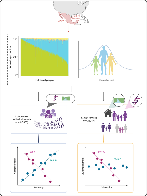
From the 140,829 participants we selected two non-overlapping subsets, a set of families (consisting of two or more genotyped siblings and zero, one or two genotyped parents; Extended Data Table 1) and a separate set of people who were not related up to the fourth degree of relatedness. Pair-wise relatedness for all samples was inferred with KING⁵², using the option –ibdseg, as described previously⁴. From the 30,450 sibling pairs identified by KING, those identified as full siblings were grouped into family units. To ensure that all pairs within a family were full siblings according to KING’s estimation, 25 people were removed. Furthermore, four people were excluded to ensure that each family had no more than two putative parents. The filtration resulted in a family dataset comprising 30,407 full-sibling pairs within 16,187 families (n = 38,274). To refine the family structure further, we incorporated parent–offspring relationships, identifying people with genotype data for both parents, resulting in 1,440 complete parent–offspring trios. Consequently, the family-based dataset comprised 39,714 people with either full siblings or two genotyped parents. The ‘population sample’ was selected from the 63,130 people who were unrelated up to the fourth degree of relatedness, excluding family set people and their parents, leading to a sample set of 52,583. Restriction to this unrelated set was done to minimize confounding due to pedigree relatedness in estimating population-level effects.

Estimation of IBD sharing among siblings

For each identified family, genome-wide IBD was estimated with snipar (single-nucleotide imputation of parents)⁵³ based on genotype array data. snipar employs a hidden Markov model to infer IBD segments shared between siblings, achieving near-theoretical accuracy and reducing IBD errors compared to KING⁵³. When running snipar, genotyping array variants were filtered based on the following criteria: minor allele frequency less than 5%, significant deviation from Hardy–Weinberg equilibrium (P < 1 × 10⁻⁴), or missingness greater than 1%. Furthermore, a genotyping error probability threshold of 4.5 × 10⁻⁴ was applied.

A comparison of estimated genome-wide IBD proportions among sibling pairs using either genetic or physical genome length is shown in Supplementary Fig. 11. For subsequent analyses, we used the realized relationships among sibling pairs estimated from snipar, with IBD defined as the genome-wide proportion of genetic map length (in centimorgans) shared.

Phenotype selection

Fifteen complex traits data at baseline were explored in the analysis, including height, weight, BMI, waist-to-hip ratio (WHR), SBP, diastolic blood pressure (DBP), high-density lipoprotein cholesterol (HDL), LDL, total triglycerides, apolipoprotein A1 (ApoA1), ApoB, HbA1c, estimated glomerular filtration rate (eGFR), an ordinal categorical variable, EA, and one disease, T2D. eGFR was calculated using the formula of the Chronic Kidney Disease Epidemiology Collaboration 2021, which considers age, sex, and creatinine plasma concentration⁵⁴. SBP and DBP were adjusted by adding 15 or 10, respectively, separately if the participants took antihypertension medication⁵⁵. EA was represented by a category variable, education (4, university or high school; 3, middle school; 2, elementary; 1, illiterate or literate), which is treated as a continuous trait in the analysis. As a sensitivity analysis we also considered a finer-grained measure of education using 14 categories (Supplementary Table 11). The inverse normal distribution function was used to derive category thresholds for the 14 categories from their cumulative probabilities, and the mean z-score for each category was calculated assuming an underlying normal distribution with several thresholds. This transformation placed the 14 ordinal EA categories on an underlying normal scale. The phenotypic correlation between the 1–4 scale and the 14-category z-score scale in the entire MCPS cohort was 0.94.

People were considered to have T2D if they reported a previous diagnosis of diabetes (diagnosed age at least 35 years) or were taking anti-diabetic medication at baseline. People who reported a diagnosis before age 35 years and were on insulin were considered likely to have type 1 diabetes and were excluded from the T2D case set. Participants without a previous diabetes diagnosis or on anti-diabetic medication and with HbA1c < 6.0% were classified as normoglycaemic controls. The American Diabetes Association uses an HbA1c threshold <5.7%⁵⁶, and therefore we used this threshold to select controls in a sensitivity analysis. Phenotype outliers were excluded if height was less than 120 cm or greater than 200 cm, weight less than 35 kg or greater than 250 kg, BMI (kg m⁻²) less than 15 or more than 60, and WHR less than 0.5 or more than 1.5. To make the effect scale comparable across phenotypes, continuous traits were adjusted for age and age² and standardized (mean 0, s.d. 1) within each sex, and outliers were further excluded according to mean ± 5 s.d. Further adjustments were applied for specific traits: BMI was residualized in the standardization for WHR, and fasting duration was residualized for HDL, LDL, total triglycerides, ApoA1 and ApoB. Stata (v.18.5) was used for phenotype data processing.

Multiple testing adjustment

To determine the statistical significance of estimated ancestry effects, we calculated the total number of independent tests and adjusted the P threshold accordingly. Each trait had three estimates (one from the population sample and two from the family sample) for each of the three ancestries, resulting in a total of nine comparisons per trait. Given that the 15 traits were correlated (Supplementary Table 12), we estimated the effective number of independent traits using the eigenvalues of the phenotypic correlation matrix⁵⁷. The estimated number of independent traits was 9.43, leading to a study-wide significance threshold of 5.89 × 10⁻⁴ (0.05/(9 × 9.43)).

Estimation of ancestry effects

For the sample of unrelated people, linear regression analyses were conducted using R (v.4.3.2) to estimate the association between ancestries and complex traits. District (Iztapalapa or Coyoacán) was included as a covariate for all traits. Sex, age and age² were included as covariates for T2D analyses. HbA1c and eGFR were analysed exclusively in the subset of non-diabetic people, defined as those without a T2D diagnosis, not taking anti-diabetic medication and with HbA1c under 6.5%⁵⁸. Furthermore, sensitivity analyses were performed, adjusting for the first seven genetic PCs or without fitting district as covariates (Supplementary Table 13). Note that only the first seven PCs were used as these PCs had normally distributed SNP loadings across the genome—a signature of population structure—as opposed to non-normally distributed loadings indicative of long-range LD^4,59.

Quantitative traits in the family data were analysed using linear mixed models, fitting individual genetic effects and shared environmental effects as random effects and between- and within-family ancestry effects (IAM, AFR and EAS) as fixed effects (Supplementary Note 1). These analyses were performed in GCTA⁶⁰ (v.1.94.3). The covariance structure between the phenotypes of siblings was modelled by fitting the estimated IBD relationship matrix and a matrix for shared environmental effects, as done previously^28,29. These models simultaneously estimate between- and within-family ancestry effects and variance components for genetic and shared environmental effects.

Ancestry association analyses were conducted with EUR ancestry specified as the reference. IAM and EUR ancestries together account for most (greater than 90% on average) genome-wide inferred ancestry in this population, and model identifiability constraints permit the inclusion of only three of the four ancestry components. Retaining IAM in the model therefore enabled a more interpretable result in this study population where genetically inferred IAM ancestry comprises the largest proportion.

Analysis of T2D

T2D was the only binary (0–1) trait and was analysed using both linear (mixed) models and generalized linear (mixed) models. The statistical software packages we used did not have an option for a generalized linear mixed model with multiple random effect and user-specified covariance structures. We did have that option for linear mixed models and used that for T2D so that on the 0–1 scale it is the same model as for the quantitative traits. For the population set, we first fitted a simple linear model using lm in R (v.4.3.2) and subsequently fitted a generalized linear model with a logit link function, using glm in R. For the family data we fitted a linear mixed model on the 0–1 scale using GCTA, as was done for the quantitative traits, and transformed the variance components to a liability scale (as implemented in GCTA), assuming a population prevalence of 15.54%, which is the prevalence in the entire MCPS population with T2D data (n = 125,042). We also fitted a generalized linear mixed model using glmer in R (lme4 package). To facilitate model convergence, age was rescaled to have a mean of 0 and an s.d. of 1. However, this implementation can only fit a single random effect with a simple covariance structure and therefore we fitted family as the only random effect.

Effect estimates on the linear (0–1) scale are therefore on the scale of prevalence, which aids interpretation. To approximate predicted prevalence of T2D in 100% IAM from the logistic multiple regression analysis on the population sample, we used \(p(x)=1/(1+For more tech updates, stay tuned to our blog.^Check back often for more exciting news!)\), where \(p(x)\) is the probability of disease given IAM ancestry proportion \(x\), \(\beta \) is the estimated coefficient from the logistic regression and \(\alpha \) is estimated as \(\alpha \approx \mathrmKeep following us for the latest insights.(K)-\beta \barCheck back often for more exciting news!\), with \(K\) the prevalence of T2D in the sample. This provides an approximation of \(p(1)-p(0)\), the counterfactual contrast of disease prevalence in 100% versus 0% IAM genome-wide ancestry proportions. Alternatively, a first-order approximation to the marginal effect on the prevalence scale is given by \({\beta }_{\mathrm{linear}}\approx \beta K(1-K)\), evaluated at the sample prevalence K.

cTIA analysis

We estimated a cTIA for height and T2D for each person in the sample of 52,583 unrelated people. For each of these traits, we used results from trans-ancestry GWAS. For height we took the set of 12,111 SNPs from a conditional and joint (COJO) SNP analysis³². For T2D, we took 1,289 independent genome-wide significant variants from Suzuki and colleagues³³. Height COJO variants and T2D GWAS variants were matched to MCPS genomes using previously TOPMED-imputed hard-call genotypes⁴ and, for each person, the cTIA was calculated by adding up the number of trait-increasing alleles, using the –score sum function in PLINK⁶¹ (v.1.9). The Ensembl Variant Effect Predictor⁶² tool was used to make annotations for the trait-associated SNPs of 12,111 COJO variants from Yengo and colleagues³² and the 1,289 independent genome-wide significant variants from Suzuki and colleagues³³. Loss-of-function variants were defined as the variants with annotation frameshift, stop gained, stop lost, start lost, splice acceptor or splice donor⁶³. A total of 314 (2 of 316 missing in the MCPS) missense and loss-of-function variants were identified for height-associated SNPs and 36 (6 of 42 missing in the MCPS) missense variants for T2D. To evaluate the association between cTIA and a specific ancestry while controlling for the effects of the other two ancestries, we conducted a partial correlation analysis using the ppcor⁶⁴ package in R. To estimate the effect of ancestry after accounting for a cTIA we fitted the latter as a fixed effect in the mixed linear model analysis of the family data. For the T2D analysis, the cTIA was scaled to have a mean of 0 and an s.d. of 1. In the sensitivity analyses, we also fitted a cTIA associated with EA, including 2,925 COJO variants identified in people of European ancestry⁶⁵.

Selection analyses

We followed the approach of Guo and colleagues³⁷. Allele frequencies for EUR ancestry were taken from the independent European population (n = 348,658) in the UK Biobank. Allele frequencies for IAM were calculated from a sample of 1,012 people in the MCPS who had an estimated genome-wide proportion of IAM ancestry greater than 99.5%. Allele frequencies were therefore estimated from people who were either of approximately 100% IAM ancestry or 100% EUR ancestry using imputed hard-call genotype data and were not affected by admixture or assortative mating within the MCPS. As both the GWAS for height and T2D were from predominantly EUR samples, we used European samples (n = 503) of the 1KG reference to calculate LD scores, applying the –ld-score and –ld-score-adj functions in GCTA⁶⁰ with a window size of 1,000 kb. SNPs from the GWAS summary statistics^32,33 were matched with those having EUR frequency, IAM frequency and LD score, resulting in 1,183,521 and 8,447,340 variants for height and T2D, respectively. The fTIA in IAM and EUR was calculated for the trait-associated 12,111 (11,778 available) COJO variants from Yengo and colleagues³² and the 1,289 (1,208 available) genome-wide significant variants from Suzuki and colleagues³³. F_ST for each of the associated variants was calculated from Hudson’s F_ST equation⁶⁶:

where \({\mathop{p}\limits^{ \sim }}_{1}\) is the estimated fTIA in IAM, \({\mathop{p}\limits^{ \sim }}_{2}\) the estimated fTIA in EUR and n_i the sample size. To generate a null distribution, control SNPs matched on fTIA in EUR and LD score were sampled from the GWAS summary statistics (excluding the trait-associated variants), and their fTIA were calculated in IAM and EUR³⁷. This was repeated 10,000 times, both for the analysis of F_ST and the analysis of the difference in trait-increasing alleles.

To correlate fTIA differences with effect sizes for the genome-wide trait-associated variants, we multiplied the square of the estimated effect size in the GWAS with expected heterozygosity (2 × fTIA × (1 − fTIA)) in EUR (Supplementary Fig. 10).

For the association between SNP rs200342067 and height, we performed linear regression analyses in the set of 52,583 unrelated people, adjusting for ancestries, age, age², sex and district.

Comparison of estimates from the population and family data

To explore concordance of the estimated ancestry effects from the family and population datasets, we used the estimated between and within-family effect sizes from the family data, predicted the population effect size (Supplementary Note 2) and then compared the predicted values with the ‘observed’ estimate from the independent population sample. The predicted value is a linear combination of the between and within-family effect size and we derived its sampling variance (and s.e.) using the reml-est-fix-varcov function in GCTA, which provides the full variance–covariance matrix of the fixed effect estimates from the mixed model analysis.

Ethics statement

Ethics approval was obtained from the Mexican Ministry of Health, the Mexican National Council for Science and Technology and the University of Oxford, UK. All participants provided written informed consent.

Reporting summary

Further information on research design is available in the Nature Portfolio Reporting Summary linked to this article.