Labelling the cellular structures with ECL probes Preparation of Ru(bpy)3 2+–N-hydroxysuccinimide-ester-labelled antibody 1 ml, 1 mg ml−1 goat anti-rabbit immunoglobulin G (IgG) antibody (Huabio, HA1002) was dialysed (Viskase, Membra-Cel MD44) overnight at 4 °C in 3 l of 0.01 M phosphate buffer saline (PBS, pH 7.6, Sigma) and adjusted to a concentration of 2 mg ml−1. Then 1 mg of Ru(bpy)2(mcbpy-O-Su-ester)(PF6)2 (Aladdin, R131404) was dissolved
Labelling the cellular structures with ECL probes
Preparation of Ru(bpy)3
2+–N-hydroxysuccinimide-ester-labelled antibody
1 ml, 1 mg ml−1 goat anti-rabbit immunoglobulin G (IgG) antibody (Huabio, HA1002) was dialysed (Viskase, Membra-Cel MD44) overnight at 4 °C in 3 l of 0.01 M phosphate buffer saline (PBS, pH 7.6, Sigma) and adjusted to a concentration of 2 mg ml−1. Then 1 mg of Ru(bpy)2(mcbpy-O-Su-ester)(PF6)2 (Aladdin, R131404) was dissolved in 50 µl dimethyl sulfoxide and added to the purified goat anti-rabbit IgG antibody immediately. The reaction mixture was incubated at 25 °C for 1 h. Subsequently, the unreacted Ru(bpy)2(mcbpy-O-Su-ester)(PF6)2 was removed using dialysis (4 °C, in 3 l PBS for 6 h, with buffer replacement every 2 h). The obtained labelled antibody was diluted with PBS to a final concentration of 1 mg ml−1 for use.
Thank you for reading this post, don't forget to subscribe!Cell culture and immunolabelling
The HeLa cells, COS-7 cells and MCF-7 cells (Shanghai Institute of Biochemistry and Cell Biology, Chinese Academy of Sciences) were cultured at 37 °C with 5% CO2 in high-glucose Dulbecco’s modified Eagle’s medium (DMEM, Gibco) mixed with 10% foetal bovine serum (FBS, Gibco) and 1% penicillin-streptomycin solution (Sangon Biotech). When reaching about 90% confluency, the cells were digested by 0.25% trypsin-ethylenediaminetetraacetic acid (trypsin-EDTA, Thermo Fisher Scientific) solution for 1 min and then transferred to sterilized indium tin oxide (ITO) coverslips. After 24 h, the transferred cells were rinsed with PBS three times and immediately fixed for 30 min at room temperature with 4% paraformaldehyde (PFA, Sangon Biotech). The excess PFA was removed by washing the samples with PBS. Then the cells were permeabilized and blocked with 1% Triton X-100 (Sigma-Aldrich) mixed with 5% bovine serum albumin (BSA, Sangon Biotech) in PBS for 1 h at room temperature. After washing, the cells were stained by rabbit anti-alpha tubulin antibody (Abcam, ab52866) with a dilution of 1:100 in 5% BSA/PBS blocking buffer overnight at 4 °C. For mitochondrial imaging, the cells were stained with rabbit anti-TOMM20 antibody (Abcam, ab186735). For CEA imaging, the cells were stained with rabbit anti-carcinoembryonic antigen CEA antibody (Abcam, ab133633). For integrin imaging, the cells were stained with rabbit anti-integrin alpha 5 antibody (Abcam, ab275977) under the same conditions. The cells were then washed three times with PBS and stained with 10 µg ml−1 Ru(bpy)32+-labelled goat anti-rabbit IgG antibody at 37 °C for 2 h. Finally, the cells were washed three times and imaged. Cell lines were authenticated using short tandem repeat analysis by the supplier. All cell lines were routinely tested and confirmed to be negative for mycoplasma contamination.
Labelling the cellular structures with CL and BL probes
Construction of mammalian expression vectors
CL and BL labelling of the intracellular targets was achieved by using a genetically encoded BRET probe (GeNL), which used NanoLuc luciferase as the donor and mNeonGreen fluorescent protein as the acceptor in this study. The only difference is that CL was applied to fixed cells, whereas BL was applied to live cells. The GeNL system was constructed according to the reference method26. All targeted sequences used for cell transfection are listed in Supplementary Table 2.
Cell culture and transfection
HeLa, COS-7 and MCF-7 cells were transfected at approximately 70–90% confluence with 0.25 μg of plasmid DNA using Lipofectamine 3000 (Thermo Fisher Scientific). After 12 h, the medium was replaced with phenol red-free DMEM for subsequent live-cell BL imaging.
ECL imaging
ITO coverslips were prepared using the reported protocol6. An inverted optical microscope (IX83, Olympus) with an oil immersion 100× objective (numerical aperture (NA) = 1.45, Olympus) was used. For large FOV imaging, an oil immersion 40× objective (1.35 NA, Olympus) was used. A 488-nm laser beam (MDL-D-488-200 mW, CNI) was delivered through a single-mode fibre and a collimator (FP5-F5AP-A, LBTEK) and then coupled into the microscope for the fluorescence excitation of the Ru(bpy)32+ probe for cross-validation. The images were captured by a water-cooled (178 K) electron-multiplying charge-coupled device (EMCCD) camera (iXon Ultra 897, Andor). The ECL images were collected under an electron multiplying (EM) gain of 500 and different exposure times (20 ms, 200 ms, 500 ms, 1,000 ms, 3,000 ms).
For ECL excitation, a three-electrode electrochemical system was used with ITO, Ag/AgCl and Pt plate (10 mm × 10 mm × 0.1 mm) as the working electrode, the reference electrode and the counter electrode, respectively. 100 mM TPrA (Energy Chemical) and 100 mM Bis-tris (Energy Chemical) in 0.01 M PBS were used as the ECL imaging buffer, respectively. An electrochemical workstation (CHI 760e, CH Instruments) was used to control the applied voltage and perform cyclic voltammetry. The excitation voltage was varied between 0.9 V and 1.8 V versus Ag/AgCl. The cyclic voltammetry scan range was between 0 V and 2 V, with a scan rate of 0.1 V s−1.
2D-ECL image sequence was acquired with the electrode surface as the focal plane and 3D-ECL image sequence was acquired in axial scanning mode with a scanning step of 200 nm starting from the electrode surface (0 µm) to the upper layer (1.6 µm) while synchronously increasing the applied voltage from 1 V to 1.8 V with a 0.1-V step. For large FOV imaging, the stage was shifted to each of the nine sub-FOVs (512 × 512 pixels, about 204 µm × 204 µm) with 20% overlap.
CL imaging
CL images were collected under an EM gain of 500 and an exposure time of 500 ms/1,000 ms. 10 μM FFz (Promega) in PBS buffer was used for CL excitation. NanoLuc first catalyses FFz to generate CL, which transfers to the proximity of mNeonGreen fluorescent protein for luminescence. An axial scanning stack with a 200-nm step was acquired here for 3D-CL imaging of mitochondria, which was subsequently concatenated into a 3D projection.
BL imaging
Live-cell imaging was conducted at 37 °C in 5% CO2 using an inverted microscope (Ti2e, Nikon) equipped with oil immersion objectives (100×/1.42 NA, Nikon; 60×/1.49 NA, Nikon) and a live-cell workstation (STXG, Tokai Hit). A 488-nm laser beam (Oxxius, L4Cc) was introduced for the fluorescence cross-validation. The image stacks were captured by the EMCCD camera. The BL images were collected under an EM gain of 500 and exposure times of 100 ms, 500 ms or 1,000 ms. The BL imaging buffer (4 μM/6 μM/10 μM FFz prepared in phenol red-free DMEM, supplemented with 10% FBS) was refreshed at a rate of 40–250 µl min−1 using a peristaltic pump (Masterflex, Ismatec Reglo ICC) during BL imaging to obtain a steady luminescence signal, while minimizing the cytotoxicity induced by substrate-generated radicals.
Cell viability evaluation
To assess the cellular impact of BL, we used an established cell physiology evaluation metric—the phototoxicity fitness time trial40. Cell viability and physiological integrity were assessed through division time, cellular diameter, mitochondrial dynamics, membrane integrity and viability assay. A continuous 24-h bright-field observation was conducted for the cell division with 4 µM FFz in the DMEM. The division time was determined by TrackMate41 (a plugin of Fiji/ImageJ). The membrane integrity was determined by a commercial dye, propidium iodide (PI, Thermo Fisher Scientific). Dead cells with compromised membrane integrity were subsequently identified and quantified by measuring the red nuclear fluorescence signals.
RIED reconstruction
Main steps of RIED
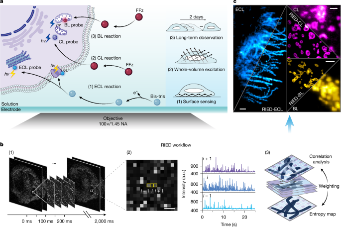
In ECL imaging experiments, strong sampling noise interferes with the effective extraction of ECL temporal fluctuations. To mitigate this, we first applied a 2D Gaussian filtering preconditioning step to the raw ECL stack, effectively suppressing high-frequency noise beyond the passband of the imaging system. Second, Fourier interpolation was performed to upsample the ECL stack along the x–y direction, recalculating the images on a finer grid. This process ensured sufficient pixel support for the subsequent resolution enhancement. Third, a pre-deconvolution step using accelerated Richardson–Lucy (RL) deconvolution was used to reduce the sampling noise and enhance the resolution12. These preprocessing steps ensured that the subsequent entropy-weighted correlation cumulant focuses on enhancing the resolution using the ECL temporal responses on a finer grid, without being affected by the noise or the spurious fluctuations. Finally, the post sparse deconvolution with dual constraints was executed as the last step to maximize the image quality and the spatial resolution (fulfilling a \(2\sqrt\text\) improvement in 3D resolution). The same RIED workflow was used for CL/BL unless otherwise specified.
Entropy-weighted correlation cumulant
Entropy was used to identify ECL emitters, which can be considered as the expected information content of the ECL photon events. The entropy value is higher if there are more photon events, which makes the pixel contain greater intensity variation and higher information content. By calculating the entropy value for each pixel, the ECL signals were effectively highlighted against the random sampling noise. Moreover, as entropy captures the spatial distribution of ECL emitters, the resulting entropy map provides a weighting scheme for correlation analysis, compensating for the spatiotemporal heterogeneity in the ECL emission. A sample in the ECL imaging system can be seen as a collection of individual ECL emitters (N) located at position rk exhibiting stochastic and independent emission behaviours, which can be described as
$$R(r,t)=\mathopFor more tech updates, stay tuned to our blog.\limits_y^h(r-Keep following us for the latest insights._y)\times _Keep following us for the latest insights.\times _(t)$$
in which h, l and w represent the PSF of the ECL imaging system, the emitter luminescence brightness and the emitter time-dependent emission events, respectively. To exploit the individual blinking characteristic of each ECL probe molecule, we calculated the correlation cumulant to deplete the pixels dominated by overlapping emitters and narrow the PSF, which can be given as
$$\beginCheck back often for more exciting news!{c}G(r)={\langle \delta R(r,t)\cdot \delta R(r,t)\rangle }_{t}\\ \,=\sum _{i,j}h(r-{r}_{i})\times h(r-{r}_{j})\times {l}_{i}\times {l}_{j}\times {\langle \delta {w}_{i}(t)\cdot \delta {w}_{j}(t)\rangle }_{t}\\ \,=\mathop{\sum }\limits_{i=1}^{N}{h(r-{r}_{i})}^{2}\times {{l}_{i}}^{2}\times {\langle {\delta {w}_{i}(t)}^{2}\rangle }_{t}\end{array}$$
in which δR(r, t) = R(r, t) − ⟨R(r, t)⟩t and ⟨∙⟩t denotes the time averaging. As the emission events of individual ECL probe molecules are independent and uncorrelated with those of the others, the correlation terms between different emitters (i ≠ j) vanish and only autocorrelation terms remain in the result. Then the spatiotemporal cross-correlation cumulant was calculated for interpolation pixels between the original adjacent pixels:
$$\begin{array}{l}{xG}({r}_{1},{r}_{2})={\langle \delta R({r}_{1},t)\cdot \delta R({r}_{2},t)\rangle }_{t}\\ \,=\mathop{\sum }\limits_{i=1}^{N}{h\left(\frac{{r}_{1}+{r}_{2}}{2}-{r}_{i}\right)}^{2}\times {{l}_{i}}^{2}\times {\langle {\delta {w}_{i}(t)}^{2}\rangle }_{t}\end{array}$$
in which r1 and r2 represent the adjacent positions of original pixels and (r1 + r2)/2 is the geometric centre of r1 and r2. The cross-correlation cumulant takes advantage of the high-contrast blinking of ECL probe molecules, filtering out the pixels dominated by overlapping emitters in an effective way. When taking the second-order correlation cumulant with zero time lag, the reconstruction results in a PSF narrowing by a factor of \(\sqrt{2}\).
Notably, although the high contrast ratio induced by ECL reactions enables considerable resolution improvement, the inherent spatiotemporal heterogeneity of the ECL probe molecules tends to introduce discontinuities in the correlation reconstruction. Therefore we introduced the Shannon entropy as a weighting factor for compensation:
$$E(r)=-\mathop{\sum }\limits_{i=1}^{n}P(r,i)\times {\log }_{2}(P(r,i))$$
in which P is the intensity probability distribution of the pixel located at position r. The entropy measures the expectation of the information content to judge whether there exist ECL emitters or not. A high entropy value indicates a dense distribution of the ECL probe molecules, which provides an emitter distribution map to weight the correlation reconstruction and compensate for the spatiotemporal heterogeneity. The entropy-weighted autocorrelation is given as:
$$E(r)\cdot G(r)=-\mathop{\sum }\limits_{i=1}^{n}P(r,i)\times {\log }_{2}(P(r,i))\times {\langle \delta R(r,t)\cdot \delta R(r,t)\rangle }_{t}$$
Also, the cross-entropy was calculated to measure the information content between the original adjacent pixels:
$$xE({r}_{1},{r}_{2})=-\mathop{\sum }\limits_{i=1}^{n}P({r}_{1},i)\times {\log }_{2}(Q({r}_{2},i))$$
in which Q is the intensity probability distribution of the neighbouring pixel. Thus, the cross-entropy weighted cross-correlation was calculated as:
$$xE({r}_{1},{r}_{2})\cdot xG({r}_{1},{r}_{2})=-\mathop{\sum }\limits_{i=1}^{n}P({r}_{1},i)\times {\log }_{2}(Q({r}_{2},i))\times {\langle \delta R({r}_{1},t)\cdot \delta R({r}_{2},t)\rangle }_{t}$$
Post sparse deconvolution
In general, to achieve the optimal spatial resolution under the Nyquist sampling criterion, the PSF must cover at least a 3-pixel-square area, ensuring continuity along the lateral axes. Furthermore, ECL emission signals are blurred by the optical system and further degraded by noise during detection, making the true signal even sparser than the recorded one. Accordingly, the continuity prior and the sparsity prior are involved in RIED to constrain the final step deconvolution to reduce the artefacts and improve the resolution and, thus, the post sparse deconvolution is given as:
$${\arg \text{min}}_{y}\{{||{\rm{E}}{\rm{C}}-{h}^{2}y||}_{2}^{2}+{\lambda }_{{\rm{c}}}R(y)+{\lambda }_{{\rm{s}}}{||y||}_{1}\}$$
in which the first term represents the distance between the result of entropy-weighted correlation EC and the recovered image y, h is the PSF of the ECL imaging system, the second and third terms represent the continuity and sparsity constraints, respectively, and λc and λs denote the weight factors to balance the image continuity and the resolution improvement, respectively.
Specifically, an optional iterative wavelet analysis step was designed to remove the out-of-focus noise in CL/BL imaging. The out-of-focus luminescence emission can be estimated by iteratively extracting the lowest-frequency wavelet bands of the entropy-weighted correlation cumulant17. The reconstructed result is therefore given by:
$${\arg \text{min}}_{y}\{{||{\rm{E}}{\rm{C}}{-h}^{2}y-{\rm{I}}{\rm{W}}{\rm{T}}{\rm{A}}({\rm{E}}{\rm{C}})||}_{2}^{2}+{\lambda }_{{\rm{c}}}R(y)+{\lambda }_{{\rm{s}}}{||y||}_{1}\}$$
in which IWTA is the iterative wavelet analysis for estimating out-of-focus noise from EC.
3D-RIED reconstruction
To achieve 3D super-resolution ECL reconstruction, RIED can be easily transformed into the 3D form. Specifically, the ECL imaging stacks at different depths were consecutively collected through synchronous control of the voltage and the imaging focal plane change. Then the preprocessing of Gaussian filtering, Fourier interpolation, pre-deconvolution and entropy-weighted correlation calculation was conducted on each ECL imaging stack at different depths to reduce the sampling noise and enhance the resolution in the x–y direction.
After that, the results of the entropy-weighted correlation obtained at different depths were concatenated into a 3D matrix. To match the resolution improvement and resolve more subtle details in the z-direction, the Fourier interpolation was used to axially upsample the 3D matrix to result in smaller axial size voxels. As a final step, the 3D sparse deconvolution approach was applied to the Fourier-interpolated 3D matrix to increase the spatial resolution.
High-throughput super-resolution reconstruction
For high-throughput large-FOV super-resolution ECL imaging, the RIED super-resolution reconstruction was performed for each sub-FOV with a temporal upsampling strategy. The Fourier interpolation was used to upsample the ECL raw images along the t-direction, which provided a finer time interval to describe the ECL blinking, resulting in a decrease in the temporal heterogeneity of the ECL emission (Supplementary Fig. 7). In the final step, we used the BigStitcher ImageJ plugin42 to stitch the super-resolution reconstruction tiles (3 × 3) to a full super-resolution image of about 0.53 × 0.53 mm2. Segmentation and curvature/orientation analyses of microtubule filaments from different mitosis phases were performed using a microtubule filament retrieval computational tool SIFNE43 with default parameters.
Simulation analysis of reconstruction fidelity under heterogeneous emission
To assess the potential reconstruction artefacts under low-photon and heterogeneous-emission conditions, we performed quantitative simulations in which two types of emission heterogeneity were explicitly defined. Luminescence yield heterogeneity, reflecting the spatially non-uniform photon output across the emitters, was modelled as a log-normal distribution η(x, y) ~ log-normal(µ, σ2). Blinking kinetics heterogeneity, describing spatially distributed on/off switching rates, was modelled as a beta distribution τ(x, y) ~ beta(α, β). Reference parameters for typical heterogeneity levels in different luminescence modalities were estimated from the experimental data, with representative values of σ = 0.6, α = β = 3 (ECL); σ = 0.3, α = β = 8 (CL); and σ = 0.2, α = β = 8 (BL). Four synthetic heterogeneity levels were then generated: low (σ = 0.1, α = β = 10), medium (σ = 0.3, α = β = 7), high (σ = 0.6, α = β = 4) and extremely high (σ = 0.8, α = β = 2). For each heterogeneity level, dual-line structures were simulated and reconstructed using RIED with different frame numbers (100, 200, 500 and 1,000 frames). Reconstruction fidelity was quantified using the peak signal-to-noise ratio (PSNR) and RSE against the ground truth. The results show that noticeable reconstruction deviations arise only under the combined conditions of extremely high heterogeneity and limited frame number. Under other conditions, including low-to-high heterogeneity levels with sufficient frames, the reconstructed structures remain largely consistent with the ground truth, with no evident artefact amplification. Given that experimental ECL, CL and BL systems in this work typically fall within the low-to-high heterogeneity range, these results suggest that RIED can recover structural features with good fidelity under standard experimental conditions.
Performance metrics
Spatial resolution
The FRC resolution and rFRC map24 were calculated using two independent frames with identical content under the same imaging conditions. These frames were obtained by splitting the raw ECL image sequence into two subsets and reconstructing them separately.
SSIM
The SSIM44 is defined as
$${\rm{SSIM}}(x,y)=\frac{(2{\mu }_{x}{\mu }_{y}+{c}_{1})(2{\sigma }_{x,y}+{c}_{2})}{({\mu }_{x}^{2}+{\mu }_{y}^{2}+{c}_{1})({\sigma }_{x}^{2}+{\sigma }_{y}^{2}+{c}_{2})}$$
in which x represents the reference image, which is the RIED reconstruction result from a 1,000-frame ECL image stack, y denotes the corresponding RIED reconstructions using ECL image stacks ranging from 20 to 800 frames, µx and µy are the averages of x and y, respectively, σx,y is the covariance of x and y, σ2 is the variance and c1 and c2 are the variables used to stabilize the division with a small denominator.
PSNR
The PSNR is given by:
$${\rm{P}}{\rm{S}}{\rm{N}}{\rm{R}}(x,y)=10\times {\text{log}}_{10}\left(\frac{mn\times {\text{MAX}}^{2}}{{\sum }_{i=0}^{m-1}{\sum }_{j=0}^{n-1}{[x(i,j)-y(i,j)]}^{2}}\right)$$
in which x represents the reference image, which is the RIED reconstruction result from 1,000-frame ECL images, y denotes the corresponding RIED reconstructions using ECL image stacks ranging from 20 to 800 frames, m and n denote the row and the column of the image, and MAX denotes the maximum pixel value of the image.
Error analysis
Error maps and quantitative metrics were calculated using the SQUIRREL framework16. The reconstruction image was convolved with an estimated Gaussian kernel (resolution scaling function) to generate a resolution-scaled image, followed by linear intensity rescaling to match the raw summed reference. A pixelwise absolute difference map was computed. Two global metrics were derived: the RSE (root mean square error between the resolution-scaled image and the reference) and the RSP.
Comparing super-resolution reconstruction algorithms
We compared the reconstruction performance against prevalent fluctuation-based methods on our ECL image stack, including SOFI13, ESI45, eSRRF14 and SACD12.
SOFI
For SOFI reconstruction, a Fourier interpolation operation was performed to upsample the ECL stack along the x–y direction, after which a second-order autocorrelation cumulant was calculated. For the 3,000-frame CL data, fourth-order autocorrelation cumulants were also computed.
ESI
Image labelled with ‘ESI’ was reconstructed through the ESI ImageJ plugin with ‘image in output’ as ‘1’ and ‘Order’ as ‘2’, and other options with the default parameters.
eSRRF
Image labelled with ‘eSRRF’ was obtained through the eSRRF ImageJ plugin by means of the temporal radiality average reconstruction, with ‘Magnification’ set as ‘2’, ‘Radius’ set as ‘5’ and ‘Sensitivity’ set as ‘1’, with other parameters remaining default.
SACD
A Fourier interpolation step was performed to upsample the raw ECL stack along the x–y direction (×2), obtaining a smaller pixel size without changing the image content. Then a 2D RL deconvolution was applied to each ECL image, improving the resolution while reducing the sampling noise. After that, a second-order autocorrelation cumulant was calculated. To match the pixel size of the RIED reconstruction, a Fourier interpolation was again used, resulting in a finer pixel grid and a larger pixel number (×2). Finally, a post-RL deconvolution was applied to the interpolated cumulant, further enhancing the resolution. For the 3,000-frame CL data, fourth-order autocorrelation cumulants were also calculated.
Sparse deconvolution
A modified iterative wavelet transform was performed on the fluorescence images estimating and removing the background noise from out-of-focus emissions. Next, a Fourier upsampling operation was conducted to provide pixel size support for the subsequent resolution enhancement. In the final step, a continuity–sparsity joint constraints deconvolution was applied on the background-removed and interpolated image, resulting in a resolution enhancement reconstruction with minimized artefacts and improved robustness.
Pre- and post-deconvolution for comparative methods
To enable fair comparisons with other fluctuation-based super-resolution reconstruction methods, ESI and eSRRF were also processed with pre- and post-deconvolution steps. The pre-deconvolution consists of Gaussian pre-filtering, Fourier interpolation (×2) and RL deconvolution applied to each frame. The post-deconvolution consists of a second RL deconvolution applied to the final reconstructed image. All other parameters were kept identical to the standard implementations of each method.
SIM for live-cell imaging
To demonstrate the biocompatibility and excellent imaging time of RIED, we conducted parallel live-cell fluorescence correlation experiments for mitochondrial imaging. A commercial HIS-SIM (CSR Biotech) imaging system was used here46, which is based on an inverted fluorescence microscope (IX83, Olympus). A 488-nm laser beam (L4Cc, Oxxius), oil objective (100×/1.5 NA, Olympus) and live-cell station (H301, OKO Lab) were used for mNeonGreen fluorescent protein excitation, signal collection and live-cell incubation (maintained at 37 °C and 5% CO2 in a humidified chamber). A scientific complementary metal–oxide–semiconductor (sCMOS; Kinetix, C15440-20UP, Hamamatsu) camera was used for recording raw data videos. During fluorescence excitation, the power of the 488-nm laser was set to 5 mW mm−2 to minimize the photodamage to live cells. Continuous acquisition of fluorescence data was conducted under an exposure time of 100 ms. Finally, the SIM images were analysed and reconstructed by HiFi-SIM47. The imaging duration was quantitatively defined as the point at which the fluorescence intensity and contrast declined to 30% and 50% of their initial values, respectively.
Mitochondrial tracking and analysis
Reconstructed long-term super-resolution BL image sequences of mitochondria were first median-filtered, followed by automatic threshold-based binarization to generate masks for mitochondrial recognition. The binarized data were then imported into the TrackMate plugin41 in ImageJ for automated tracking. The mask detector module was used to identify mitochondria from the predefined binary regions, allowing localization of the irregular subcellular structures. Mitochondrial linking was realized using the Simple LAP tracker. The resulting trajectories, containing temporal coordinates and instantaneous velocities, were exported for the subsequent analysis of mitochondrial counts, diameter and velocity.
For intercellular mitochondrial transfer tracking, the manual tracking mode was used. Trajectories were recorded during the full transfer process and both before and after the event could be clearly observed. Cell segmentation was performed using the Cellpose 4.0 generalist algorithm48 and further refined by analysing the mitochondrial motion direction and origin. The extracted trajectory data, including time, position and velocity, were used for the subsequent transfer mode analysis. Mitochondrial transfer behaviour was quantified by calculating the time-dependent MSD. For each trajectory, the MSD at a time lag τ was computed using:
$${\rm{M}}{\rm{S}}{\rm{D}}(\tau )=\langle [x(t+\tau )-{x(t)]}^{2}+{[y(t+\tau )-y(t)]}^{2}{\rangle }_{t}$$
To minimize the statistical uncertainty owing to the reduced sampling at large time lags, the analysis was restricted to the first 25% of the total trajectory duration. To determine the diffusion mode, the anomalous diffusion exponent (α) was derived by fitting the MSD curves to a power-law model:
$${\rm{M}}{\rm{S}}{\rm{D}}(\tau )=4\times D\times {\tau }^{\alpha }$$
where D denotes the propotionality factor determining the magnitude of MSD. Linear regression was performed on the log–log-transformed data. All computational analysis and curve fitting were implemented using MATLAB.
Reporting summary
Further information on research design is available in the Nature Portfolio Reporting Summary linked to this article.
{For more tech updates, stay tuned to our blog.|Keep following us for the latest insights.|Check back often for more exciting news!}