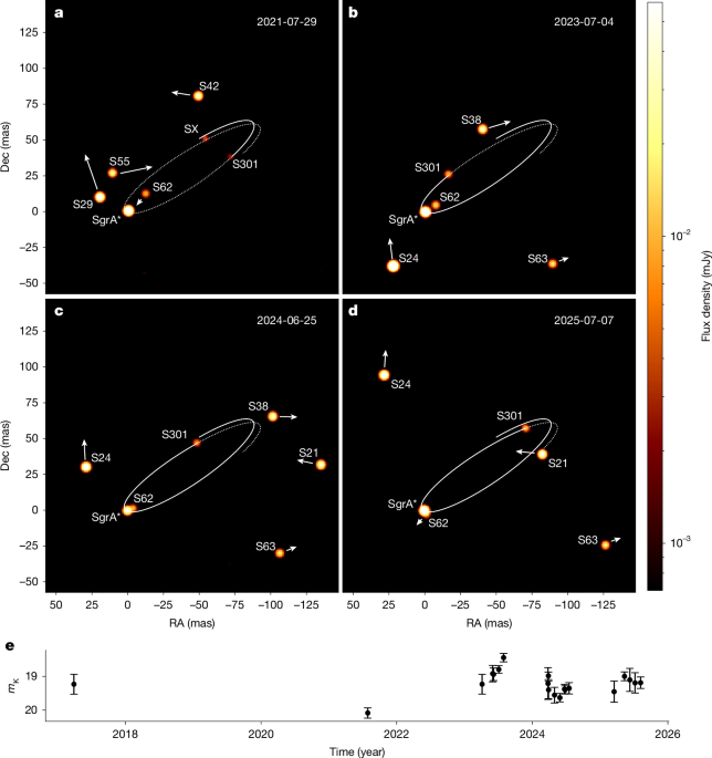
Details of observations

Our observations, from which we inferred S301, comprise 19 datasets spanning more than 8 years. We first noted S301 in 2023, when pointing directly to Sgr A*. Given the position of the star close to Sgr A* and its large proper motion, it was clear that it might be on a tight orbit, and we followed up with dedicated observing campaigns over the course of the next years. We summarize the data used for this work in Extended Data Table 1.

Based on the orbital coverage from 2023 to 2025, we were able to trace S301 back in time and identified two previously acquired datasets in 2017 and 2021, in which the star should be present. For this, we fit a preliminary orbit to the 2023–2025 data and used samples from a Markov chain to predict where the star should be in 2021. The dataset in 2021 was acquired during an observation that involved multiple other pointings in the GC to create a mosaic of the central about 200 × 200 mas (ref. ²²). This particular pointing was affected by bad seeing conditions, however, and we apply stricter cuts and accept as a post-processing step only fringe-tracking ratios of 90% for the individual detector integrations, effectively discarding data with low coherent flux. This procedure led to the inference of S301 in this particular epoch, close to the predicted position (Extended Data Fig. 3, left).

With that position in hand, we repeated the orbit fit and used the updated Markov chain to predict the S301 position in 2017. The 2017 data were acquired as part of the monitoring of the motion of the star S2, an object around five magnitudes brighter than S301. The dataset consists of individual exposures across five consecutive nights in March 2017, partially recorded in split-polarization mode. In the image reconstruction of this dataset, we treat both polarizations in polarized exposures as individual measurements and combine them with the unpolarized data. Again, S301 is found close to the predicted place (Extended Data Fig. 3, right).

Highest-resolution, deep images of the central 800 au

The high-angular-resolution, high-fidelity images of the GC are reconstructed from GRAVITY data, an example of which is shown in Extended Data Fig. 1 with the image reconstruction tool GRAVITY-RESOLVE (G^R)²². This code is designed to reconstruct stars in the GC that appear to GRAVITY as unresolved point sources and, in particular, to find faint, yet undiscovered stars. G^R is based on a hierarchical forward model that incorporates the instrument response of GRAVITY, including both optical aberrations and the spectral transmission within the beam combiner, as well as a statistical model of the GC. The intrinsic multitude of degrees of freedom of an image is tamed with Bayesian inference, in which the statistical model of the GC provides the previous information. With G^R, we exploit supreme imaging resolution of ≃ 1.7 mas of GRAVITY and its phase-referencing abilities, which allow for high contrast images and routine mosaicking as pioneered in radio interferometry (F. Mang et al., manuscript in preparation).

The individual positions of S301 over time, as shown in Fig. 2, were inferred in a first step from imaging. We initialized the model in G^R by invoking all known, bright sources within the field of view. Positions and fluxes of the stars and Sgr A* are constrained by previous distributions that reflect current knowledge. We applied G^R a total of 10 times to the same dataset with varying initial random seeds. Tentative faint sources that may appear in the image of individual reconstructions are accepted only when they are inferred in at least 5 out of 10 reconstructions. Their corresponding positions in the image grid are then referenced to Sgr A* and subsequently averaged.

Astrometric errors

The uncertainties of the newly inferred sources are derived from the scatter over the different runs, also taking into account the finite resolution of the pixel grid. This is an improvement over²² where the errors were simply approximated by the size of the pixels in the image. If the same faint source is inferred in the same pixel for the 10 individual runs, the corresponding standard deviation is zero, albeit unphysical. Hence, the discretized position space needs to be considered when stating errors on astrometry. Instead of quantifying the error based on the number of same-pixel inferences in a set of detections, we opt for a general approach, which may be conservative, but prevents an underestimation of errors. We derive a discretization error by calculating the root mean square error for a single pixel within the image for both directions, right ascension and declination, independently. Considering a pixel size of 0.8 mas per pixel, this evaluates to about 207 μas and represents the statistical uncertainty in astrometry originating from the pixel grid in G^R images. This value acts effectively as a noise floor.

Fitting of GRAVITY data

Apart from imaging with G^R, we apply two other tools to analyse GRAVITY data. These methods serve to fit individual stars, that is, parameterized point sources, foremost to determine their astrometry and photometry. They allow for a crucial cross-check whether S301 is inferred at the same position with a comparable photometry as with the image reconstruction. Both fitting tools are separately implemented in different programming languages.

In a first step, every GRAVITY exposure is fit separately to infer the variable flux of Sgr A*, equivalent to determining a light curve over time. Both inferred fluxes and positions of Sgr A* and other bright, known sources then provide the starting values for a subsequent combined fit. For S301, the values from the imaging code are used as starting values. S301 is inferred by both methods at the same position as with the imaging code, within statistical errors.

Although the fitting codes yield the same positions for S301 as G^R, it would be de facto impossible to find a star such as S301 using just a fitting code. The fitting essentially returns a local minimum, whereas the imaging efficiently explores the full parameter space.

Imaging with CLEAN

We also inferred S301 with a more classical imaging routine, namely, CLEAN (Extended Data Fig. 2). For that, we first CLEANed on Sgr A* in the individual exposures to capture its variability. The corresponding coherent flux is then subtracted from the data before combining the data and running a deeper CLEAN, allowing to infer fainter sources, such as S301 and S62.

Best-fit orbit

We fit the astrometric positions of S301 in the same way as we did for the S2 data in ref. ⁸, taking into account Rømer delay and the 1PN correction of the motion due to the Schwarzschild nature of the gravitational potential. Relativistic Doppler effect and gravitational redshift do not matter as they only affect radial velocity measurements, which we currently do not have. This lack also results in an ambiguity in the 3D orientation of the orbit. The two viable orbit solutions to the proper motion of S301 are given in Extended Data Table 2 (angle conventions follow ref. ⁴) and leave the semi-major axis, eccentricity and time of periastron unchanged within errors. In principle, the Rømer delay could break the ambiguity²³, but does not yet for the limited phase coverage of S301. The orbit stands out compared with other S-stars. For an illustration, see Extended Data Figs. 6 and 7. The high eccentricity of S301, combined with the small value of the semi-major axis, makes S301 an outlier with the smallest value of r_p = a(1 − e). Also note that the orbital plane of one of the two possible solutions agrees to within 3° with the inner clockwise disk of young, massive stars in ref. ³².

Measuring the spin of Sgr A* with S301

The orbit-averaged Lense–Thirring effects for the in-plane and out-of-plane major axis precession are, respectively,^33,34

where ξ is the inclination between spin axis and orbital angular momentum, and λ is the position angle of the projection of the spin axis onto the orbital plane. For S301, the in-plane contribution per revolution amounts to 0.11°χ cos ξ .

To assess how S301 probes the spin of Sgr A*, we perform a mock data analysis combining current and simulated future observations. We construct synthetic astrometric and radial-velocity datasets extending the existing measurements with simulated observations between 2026 and 2035, using the values of the orbital parameters given in Extended Data Table 2, with mass and distance of Sgr A* from ref. ⁵. We optimistically adopt χ = 1 and an orientation approximately aligned with the stellar orbital angular momentum. In this case, the Lense–Thirring effect produces mainly in-plane precession and little precession of the orbital plane. The resulting mock data are fitted to test whether the spin parameters can be recovered. We assume a realistic astrometric precision of 100 μas (as expected for the final performance of GRAVITY+) and 1 km s⁻¹ accuracy on the radial velocity as reachable with future ELT/MICADO observations. A sampling of 10 data points per year until 2035, with 10 additional data points around pericentre, would yield a spin constraint with an uncertainty on χ of <0.2 (Fig. 3c), equivalent to a >5σ detection of χ = 1 compared with the non-spinning (χ = 0) case. In Extended Data Fig. 9, we show the dependence of the significance of the spin detection in our simulations as a function of orientation of the black hole spin. The maxima of significance correspond to alignment and anti-alignment of the spin and orbital angular momentum, whereas the minima correspond to alignment of the spin along the semi-major axis of the orbit. A more detailed discussion is provided in another study (K.A.E.D. et al., manuscript in preparation). Also, we note that future robust spin constraints will require modelling up to 2PN (second post-Newtonian) order to avoid systematic biases at low spins.

Spectral type, mass and age of S301

Given the magnitude m_K = 19.3 ± 0.3 and assuming an extinction of 2.42 (ref. ³⁵) and a GC distance of R₀ = 8.3 kpc (ref. ²³), S301 has an absolute K magnitude of about 2.28. It is too faint to be a giant, but it instead is compatible with being a main-sequence star. Its spectral type then is a late A-type or an early F-type star (see also figure 2 in ref. ³⁶), which means its colour index is V − K = 0.6 (ref. ³⁷). With an absolute V magnitude of 2.88, it has L = 5.5 L_⊙ and a spectral type of F1.5, corresponding to a mass of just below 1.5M_⊙. Alternatively, its mass can be estimated to be between approximately 1.1M_⊙ and 1.5M_⊙, depending on the age of the star, with younger ages corresponding to larger masses.

We infer the possible ages and masses of this star, using the observed brightness and the MIST^38,39,40 isochrones (MIST v.1.2 tracks with Ω/Ω_crit = 0.4 and solar metallicity). Specifically, we identify evolutionary points at which the track magnitude crosses the inferred absolute magnitude. The stellar ages and masses for these points are shown as a solid, blue line in Extended Data Fig. 8. Note that the MIST tracks do not include the K band magnitude, and we use the JWST F210M magnitude as a proxy.

To test the robustness of our results, we repeat this analysis with the K band magnitude from PARSEC isochrones (v.1.2S; refs. ^{41,42,43,44,45}) and show the possible ages and masses in Extended Data Fig. 8 (dashed, orange line). We note that unlike MIST, the PARSEC tracks do not include stellar rotation. Nonetheless, the results are in excellent agreement with the stellar mass ranging from about 1.1M_⊙ to 1.5M_⊙, depending on the age of the star.

Tidal effects

A previous study⁴⁶ suggests that tidal effects prevent observations of Kerr effects around Sgr A*. However, they consider stars 10M_⊙ or heavier. S301 is sufficiently small so that these tidal effects are negligible. The energy input per orbit can be estimated, using the ref. ⁴⁷ formalism

where r_p is the pericentre distance, R_⋆ is the stellar radius, m_⋆ is the stellar mass and T₂ is the tidal coupling constant. Here, we include only the leading-order quadrupole term. We estimate the tidal coupling constant using the fits from ref. ⁴⁸, assuming an n = 3 polytrope. Note that these fits extend only to η = 10, and we extrapolate them using the logarithmic slope there. Thus,

for η ≥ 10. This yields \(\delta E\approx 1{0}^{-16}G{m}_{\star }^{2}/{R}_{\star }\). It would take an order of 10¹⁷ years for tides to inject an order of unity fraction of the energy of the star. Therefore, tidal heating can be neglected at the current orbit of the star.

Comparison with previously claimed short-period stars

Over the past 5 years, several short-period stars with orbital periods as low as 4 years were claimed to have been discovered by one team using adaptive-optics based imaging techniques^49,50, thus at a resolution 15 times worse than the GRAVITY data. Safely, we can exclude that the objects in ref. ⁴⁹ named S4711 and S62 (different from the star our team calls S62; see ref. ⁵¹), and that have similar orbital periods as S301, are actually S301:

• The eccentricity of S4711 with e = 0.768 is considerably less than that of S301, and the claimed orbit has a different projection on sky, extending towards the East.

• Although S62 features a comparable eccentricity of e = 0.976, the claimed orbit revolves anticlockwise, unlike S301.

Apart from this, none of the other claimed stars have orbital elements similar to the ones of S301. Hence, S301 is newly discovered.

Furthermore, it is worth noting that the limiting magnitude of m_K ~ 20 inferred from the GRAVITY observations and reported here should have allowed us to easily detect any of the claimed discoveries if covered in our exposures. In none of our reconstructed images, we have detected a significant contribution of flux beyond background noise that we could attribute to the claimed stars.

Newtonian perturbations of the spin measurement

The simulations for the spin measurement assume that S301 orbits an isolated Kerr black hole in the absence of external perturbations. As noted in ref. ³³, gravitational perturbations from a population of stellar-mass black holes, expected to form a power-law-density stellar cusp around Sgr A*, can induce orbital precession comparable in magnitude to the Lense–Thirring effect, thereby complicating the measurement of the spin. Recent constraints from ref. ²⁹ limit the extended mass within the central 10 mpc to ≲1,200M_⊙. To assess the impact of a realistic perturber population, following ref. ⁵², we performed N-body simulations of S301, including a cluster of 60 stellar-mass black holes of 20M_⊙ each, distributed within 10 mpc of Sgr A* according to a density profile ρ(r) ∝ r⁻². Considering 100 independent realizations of the initial conditions, we find that the cluster induces an average orbital-plane precession per orbital period of \(0.6{5}_{-0.56}^{+0.36}\,\text{arcmin}\). This contribution is typically sub-dominant compared with the Lense–Thirring precession for moderate-to-high dimensionless spins and favourable orientations of the black-hole spin relative to the orbital angular momentum. Importantly, the Lense–Thirring effect is concentrated near pericentre, whereas perturbations from a granular stellar background tend to produce their largest observable deviations near apocentre^52,53. This phase separation, together with the distinct temporal signatures of the two effects, offers a promising avenue to disentangle the relativistic spin signal from stellar perturbations and thereby enable a robust measurement of the MBH spin.

In an extreme case in which all the mass (allowed by S2 observations) is concentrated within the orbit of S301 in a disk and in which the orientation of the orbit is a few degrees from the disk, the nodal precession due to the disk might be larger, by up to an order of magnitude, than the Lense–Thirring precession. However, for most orientations and for less extreme mass distributions, the Newtonian effect of this mass on the nodal precession is expected to be one or two orders of magnitude smaller than the Lense–Thirring effect.

A Hills origin for S301

For the Hills mechanism^{30,54,55,56,57,58}, one of the binary components is captured at a semi-major axis of

where f₁ ≈ 0.5 for circular, equal mass binaries⁵⁹. The captured star inherits the pericentre of the orbit of the binary around the MBH, and so the binary separation must be no more than a factor of few times \({({M}_{{\rm{MBH}}}/{m}_{{\rm{bin}}})}^{1/3}{a}_{{\rm{bin}}}\) (the characteristic binary tidal disruption radius). Thus, the eccentricity of the captured star will be

where f₂ is at most a factor of order unity. The expected distribution of f₂ and hence of e_cap will depend on the distribution of binary properties (for example, the mass ratio, inclination, internal eccentricity) and the pericentre distribution of disrupting binaries. A recent study⁶⁰, simulated binary disruptions in the GC for an observationally motivated binary population, assuming a full loss cone and an isotropic inclination distribution. For captured stars with semi-major axes between 2 × 10⁻³ pc and 4 × 10⁻³ pc and masses between 1.3M_⊙ and 1.7M_⊙ the eccentricities ranged between 0.97 and 0.996 (5th–95th percentile) with a median eccentricity of 0.985. Thus, binary disruption would naturally explain the observed eccentricity of the star.

The measured semi-major axis constrains the pre-disruption binary. For nearly equal masses, the Hills mapping gives \({a}_{{\rm{cap}}}\approx \frac{1}{2}\) \({({M}_{{\rm{MBH}}}/2{m}_{* })}^{2/3}{a}_{{\rm{bin}}}\) (ref. ⁵⁹). Identifying a_cap ≃ a and adopting m_* ≃ 1.3–1.7M_⊙ yields a pre-disruption separation a_bin ≈ 0.05–0.2 au, corresponding to orbital periods P_bin ≈ 5–20 days. We find a similar range of progenitor semi-major axes in the simulations of ref. ⁶⁰, with an observationally motivated mass ratio distribution.

These compact binaries are common among F-type stars³¹ and are expected to be tidally circularized and nearly synchronized. If S301 was initially synchronized, its spin period at capture would have been comparable to P_bin, implying an equatorial rotation velocity v_rot ≈ 20–70 km s⁻¹ for R_* ≃ 1.3–1.7R_⊙. High-resolution spectroscopy with ELT/MICADO might therefore provide a direct, testable prediction of the Hills-binary origin using a measurement of \(v\sin i\).

Hills events simultaneously populate the innermost S-star cluster and the halo hyper-velocity star population. For Hills disruption rates of order \({\dot{N}}_{{\rm{H}}{\rm{i}}{\rm{l}}{\rm{l}}{\rm{s}}}\approx 1{0}^{-5}-1{0}^{-4}\,{{\rm{y}}{\rm{r}}}^{-1}\), simple steady-state arguments suggest that we expect of a order of a few S301-like stars on similarly relativistic orbits at any given time. The Hills disruption rate is supported by both the observed number of hyper-velocity stars in our galaxy⁶¹ and theoretical estimates as well as the observed tidal disruption rate in other galaxies. With roughly 10% of them having the right separation range to produce S301-like orbits (see equation (4) above), we take the formation rate of stars on S301-like orbits to be \({\dot{N}}_{S301}\approx 1{0}^{-6}\,{{\rm{y}}{\rm{r}}}^{-1}\). Given the collisional lifetime of more than 10⁸ years (Extended Data Table 3), we expect in steady state about a hundred stars with such an orbit. Most of them are likely solar mass stars, and hence still too faint to be detected. Further analysis of the observed coverage and current sensitivities of GRAVITY+ is needed to assess if this estimate is consistent with only one S301-like object detected so far; and continued GRAVITY+ monitoring and future ELT observations may therefore reveal a population of faint, low-mass S-stars deep in the potential well, enabling ensemble constraints on the spin of Sgr A* and on the distribution of stellar and remnant perturbers in the innermost approximately 10⁻² pc.

Dynamical time scales for S301

In this section, we will estimate the time scales for the orbital relaxation and collisions for S301.

Relaxation times

Relaxation is the dynamical evolution of objects due to perturbations from their environment. In the GC, relaxation can be subdivided into resonant and non-resonant parts. Resonant relaxation corresponds to the evolution of stellar orbits due to coherent torques from the background. This can lead to rapid evolution of angular momentum. On longer time scales, non-resonant (two-body) relaxation evolves the orbital energy due to uncorrelated two-body encounters (see ref. ⁶² for a review).

The two-body relaxation time scale is approximately (see equation 5.61 in ref. ⁶³)

where \(\sigma \approx \sqrt{GM/(1+\gamma )/r}\) is the one-dimensional velocity dispersion, n is the number density (with power-law index −γ), and ⟨m²⟩ is the second moment of the mass function. Owing to the quadratic mass dependence, the most massive species (namely, stellar mass black holes) often dictate this time scale.

We follow ref. ⁶⁴ to estimate the background density profile. We model the background as two species: 10M_⊙ black holes and 1M_⊙ stars. This is a reasonable approximation for modelling relaxation in an evolved galactic nucleus and has been used extensively in the literature⁶³. The stars are initialized with a Nuker density profile⁶⁵, namely,

with γ = 1.5, α = 2 and β = 5. The density normalization is set by the total mass: 2.5 × 10⁷M_⊙ and 2.5 × 10⁵M_⊙ for the stars and black holes, respectively. The central MBH starts at 4.15 × 10⁶M_⊙ and grows to 4.27 × 10⁶M_⊙ by consuming stars and black holes. The profile is allowed to relax for 10 Gyr, such that the final density profiles are not too sensitive to the initial conditions. In the end, the total mass within 0.01 pc is approximately 1,200M_⊙, consistent with the latest constraints on the enclosed mass within the apocentre of S2 (ref. ²⁹). Furthermore, the final stellar density at 1 pc (approximately 9 × 10⁴M_⊙ pc⁻³) is comparable to observational estimates⁶⁶.

The following power-law fits approximate the final density profile between about 10⁻⁴ pc and 0.01 pc:

Combining equations (6) and (8), we find that the two-body relaxation time scale at the semi-major axis of S301 (3.3 × 10⁻³ pc) would be about 9 × 10⁸ years.

To estimate the angular momentum relaxation time, including resonant relaxation, we follow ref. ⁶⁷ (and the references therein). In particular, we use their software, JuDOKA (https://github.com/KerwannTEP/JuDOKA), to compute diffusion coefficients (D_jj) as a function of eccentricity and semi-major axis for the density profiles in equation (8).

The angular momentum relaxation times can then be estimated using

where j is the angular momentum normalized to the circular angular momentum at the same energy. The top and bottom rows corresponds to the time scales without and with resonant relaxation, respectively. We find that both t_rx,j(NRR) and t_rx,j(RR) are about 3 × 10⁷ years for S301, indicating that resonant relaxation is unimportant for this star. This is expected, because of the short Schwarzschild-precession time scale of the star. In other words, the star lies within the Schwarzschild barrier, in which rapid precession suppresses the build-up of coherent torques⁶⁸.

Alternatively, t_rx,j(NRR) ≈ j²t_rx, which gives results that are consistent with equation (6).

Collision time scales

The mean time between collisions for a single target star is

where n is the local number density of potential impactors, v_rel is the typical relative velocity, and Σ is the collisional cross section. For a star of radius R_⋆ and mass m_⋆ colliding with objects of mass m_imp and radius R_imp, the cross section including gravitational focusing is

In the case of S301, m_⋆ ≈ 1.5M_⊙ and R_⋆ ≈ 1.4R_⊙. Then, from equations (8) and (11), the local collision time scale would be about 2.0 × 10⁹ years for stellar-mass black holes and about 2.1 × 10⁸ years for stars.

Uncertainties, caveats and other effects

The relaxation and collision time scales we estimate above are local. In principle, the interactions at pericentre can significantly shorten the energy relaxation and collision time scales. A naïve orbit average with the background profile in equation (8) would suggest a reduction at the order of magnitude level. In practice, fewer than one scatterer is expected at the pericentre of S301 for our assumed density profiles, so the local time scales are more realistic.

Our time scale estimates implicitly assume stars are evolving through a localized diffusion process. In reality, angular momentum and energy perturbations from a handful of massive perturbers exhibit a heavy power-law tail, such that orbital evolution would be dominated by large, non-local jumps that can speed up the orbital evolution⁶⁹.

Summary of timescales

There is a clear timescale hierarchy at the radius of S301, with T_orb ≪ T_SP ≪ T_LT ≪ T_Vec-RLX ≪ T_coll, T_Sca-RLX ≪ T_GW (Extended Data Table 3), which allows identifying the processes that are relevant for the orbit evolution of S301.