Torque and changes in the LOD

An axial torque Γ_z acting on the mantle causes a change in its rotation rate (ΔΩ_m) according to

in which C_m = 7.13 × 10³⁷ kg m² is the axial moment of inertia of the mantle. ΔΩ_m corresponds to a change in the LOD (ΔLOD)

in which Ω_o = 2π/86,400 s⁻¹ is the reference mantle rotation rate based on a 24-h day length. The equivalent torque causing the observed ΔLOD can therefore be reconstructed from

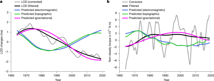
The decadal ΔLOD (grey line in Fig. 1) between 1964 and 2019 are obtained after removing the LOD contributions from the atmosphere, oceans, lunar tidal friction, glacial isostatic adjustment and barystatic processes at Earth’s surface (Extended Data Fig. 7). The multidecadal ΔLOD (black line in Fig. 1) are obtained by applying a third-order low-pass Butterworth filter with a cut-off period of 30 years to the decadal ΔLOD signal (Extended Data Fig. 8). More details on these operations are provided in the Supplementary Information.

We build predictions of ΔΩ_m (and ΔLOD) from

by numerically integrating in time from 1964 to 2019 forward models of the torque from surface forces at the CMB (Γ_cmb) and the gravitational torque from the inner core (Γ_g). We consider two different sources of Γ_cmb, electromagnetic and topographic coupling. Multidecadal ΔLOD result from fluctuations in the torque on the mantle about a mean balance^12,42,44. To focus on these, we subtract a temporal mean from all of our predictions of gravitational, electromagnetic and topographic torques.

Electromagnetic torque

The axial electromagnetic torque can be written as a surface integral over the (assumed spherical) CMB as^4,5,6

in which r_c = 3,485 km is the radius of the core, μ is the magnetic permeability of free space, B_r and B_ϕ denote the radial and azimuthal components of the magnetic field, respectively, and dS is a surface element, θ is co-latitude and ϕ is longitude. Predictions of the temporal variations of Γ_em depend on models of how B_r and B_ϕ change with time at the CMB.

The magnetic field at the CMB can be decomposed as \({\bf{B}}=\nabla \times \nabla \times {\mathcal{S}}{\bf{r}}\,+\) \(\nabla \times {\mathcal{T}}{\bf{r}}\), in which r is the radial vector and \({\mathcal{S}}\) and \({\mathcal{T}}\) are poloidal and toroidal scalar fields, respectively. B_r only involves \({\mathcal{S}}\), whereas B_ϕ involves both \({\mathcal{S}}\) and \({\mathcal{T}}\). Consequently, we can separate Γ_em into its poloidal and toroidal contributions to B_ϕ (refs. ^5,6).

The poloidal part of Γ_em can be reconstructed directly from magnetic field models built from observations. Such models provide time-dependent maps of \({\mathcal{S}}\) at the Earth’s surface, which are down-continued to the CMB. For a thin layer of conducting mantle material above the CMB with conductance G, the poloidal torque is^5,6

in which \({g}_{l}^{m}\) and \({h}_{l}^{m}\) are the Gauss coefficients of the field model (with l and m the spherical harmonic degree and order, respectively), \({\dot{g}}_{l}^{m}\) and \({\dot{h}}_{l}^{m}\) are their time derivatives and r_e = 6,371 km is Earth’s radius.

The toroidal part of Γ_em is given by

in which \({\mathscr{T}}\) includes contributions from the diffusion of the toroidal field at the top of the core into the conducting mantle and from the advection of the radial field by the flow v tangential to the CMB. We assume that the latter contribution dominates (see ref. ⁶), in which case we can write

in which \({L}^{2}=-[\frac{1}{\sin \theta }\frac{\partial }{\partial \theta }\left(\sin \theta \frac{\partial }{\partial \theta }\right)+\frac{1}{{\sin }^{2}\theta }\frac{{\partial }^{2}}{\partial {\phi }^{2}}]\) is the angular momentum operator and ∇_H is the surface gradient. Evaluation of this torque requires both a time-dependent model of the magnetic field (to evaluate B_r) and a time-dependent model of tangential flow v at the CMB. Models for v, in turn, are built such that they are compatible with the observed secular variation of the magnetic field¹⁶.

The total electromagnetic torque Γ_em is the sum of \({\varGamma }_{{\rm{em}}}^{{\rm{S}}}\) and \({\varGamma }_{{\rm{em}}}^{{\rm{T}}}\) and is proportional to the mantle conductance G, which we leave as a free model parameter to be determined. We write G = K_emG_ref, in which G_ref is a reference conductance set equal to 10⁸ S. For given magnetic field and flow models, the strength of the electromagnetic torque scales with the dimensionless conductance K_em.

Our predictions of Γ_em are based on the magnetic field model COV-OBS.x2 (ref. ⁵¹) and the probabilistic core flow model from ref. ¹⁷. These predictions are shown in Extended Data Fig. 2 and lead to multidecadal ΔLOD predictions that are broadly reversed compared with that observed (Fig. 1). The poor ΔLOD match may be because core flows are not sufficiently well resolved. Indeed, core flow models may be designed such that, as well as matching the observed secular variation, they also generate an electromagnetic torque that matches the observed ΔLOD (refs. ^6,7). The required flow adjustment tends to be small. However, although this small adjustment is not in conflict with the secular variation, it is also not required by it. Synthetic tests using numerical dynamo models show that the large-scale core flows retrieved from the secular variation contribute the most and provide an adequate prediction of the electromagnetic torque⁴⁸. This suggests that the electromagnetic torque prediction built from large-scale core flows should be broadly correct and that the mismatch with the observed ΔLOD of Fig. 1 indicates instead that electromagnetic coupling at the CMB is not the dominant multidecadal torque on the mantle. Synthetic tests⁴⁸ also suggest that the small length scales of the CMB magnetic field (l > 13), inaccessible from observations, may contribute to about a third of the total electromagnetic torque. Our reconstruction of the electromagnetic torque may then be underestimated, contributing to an overestimate in our recovered value of G.

We assume a uniform conductance G in the mantle. Although the bottommost region of the mantle (the D″ region) is most likely heterogeneous, and electrical conductivity is expected to vary with geographic position, the precise way in which it does is unknown, so the simplest approach is to assume a uniform G. Using a non-uniform G can modify the time history of the electromagnetic torque⁵² and can thus alter our inversion results for the best-fit torque parameters. However, we consider it unlikely that the geometry of G could reverse the sign of Γ_em and account for most of the multidecadal ΔLOD on its own.

Topographic torque

The topographic torque Γ_top results from the dynamic pressure associated with core flows acting on the CMB topography. Recent modelling efforts^37,38,39 focus on the perturbation in the pressure field that is induced by the deflection of a mean tangential flow by CMB bumps in a stratified fluid with buoyancy frequency N and permeated by a magnetic field of strength B₀. The axial component of Γ_top can be written as

in which T_ϕ is the azimuthal stress on the CMB. Idealized models of T_ϕ can be developed for a steady and uniform azimuthal flow v_ϕ acting on a localized region of the CMB with a periodic topography of wavelength ℓ and amplitude h. The model in ref. ³⁹ relates T_ϕ to v_ϕ as

in which \({\rm{sign}}({v}_{\phi })=\frac{{v}_{\phi }}{\parallel {v}_{\phi }\parallel }\),

and ρ is the fluid density, η is the magnetic diffusivity and F(θ) is a function of co-latitude that takes into account the projection of the Coriolis force with the normal to the boundary (Extended Data Fig. 9). The parameter \({\mathcal{D}}\) has units of kg m^−3/2 s^−3/2 and incorporates a collection of physical parameters that influence the torque. Some of these parameters (ρ, η, B₀) are reasonably well known, but N is not, and we lack a detailed model of the CMB topography, so h and ℓ are also not well constrained. To take into account different possible values of \({\mathcal{D}}\), we write it as \({\mathcal{D}}={K}_{{\rm{top}}}{{\mathcal{D}}}_{{\rm{ref}}}\), in which K_top is a dimensionless parameter and \({{\mathcal{D}}}_{{\rm{ref}}}\) is a reference value of \({\mathcal{D}}\) set equal to 1 kg m^−3/2 s^−3/2. The topographic torque from equation (9) can then be written as

The time history of Γ_top depends on the time history of v_ϕ. For a given flow model at the CMB, K_top modulates the amplitude of the topographic torque and is a parameter left to be determined. Its numerical value provides a constraint on N for the chosen values of h and ℓ (Supplementary Information).

Predictions of Γ_top based on the flow model in ref. ¹⁷ are shown in Extended Data Fig. 2. By itself, Γ_top does not generate the multidecadal ΔLOD that match observations (Fig. 1). Notably, the Γ_top model that we used is highly idealized; it is based on a steady and uniform flow at different points of the CMB, whereas the true flow is time-dependent and laterally varying. Moreover, we assume for simplicity that \({\mathcal{D}}\) is uniform but it probably has lateral variations. Allowing \({\mathcal{D}}\) to vary with position at the CMB would change the time variations of this prediction. However, the general trend of Γ_top follows that of Γ_em and illustrates that, to the first order, both of these torques depend on the fluctuations of the large-scale v_ϕ flow at the CMB; when v_ϕ is generally westward (eastward) compared with its mean time average, the tangential stress on the CMB from either electromagnetic or topographic coupling is also westward (eastward).

Gravitational torque

The gravitational torque on the mantle Γ_g is given by¹¹:

in which Γ is a strength factor and α is the longitudinal angle of the degree 2 order 2 (long equatorial axis) topography of the inner core with respect to the gravitational potential imposed by mantle mass anomalies. The evolution of α depends on the bulk axial angular rotation angle φ of the inner core (related to the differential inner core angular velocity Ω_i by \(\frac{{\rm{d}}\varphi }{{\rm{d}}t}={\varOmega }_{{\rm{i}}}\)) and the viscous relaxation time τ for the ICB topography to realign with its equilibrium shape,

We use a time history model of φ based on the seismic reconstruction from ref. ¹³ (Extended Data Fig. 1). Predictions of Γ_g depend on the time history of α, which is computed by integrating numerically equation (14) for our model of φ and a given choice of τ. Note that equation (14) describes the change in α with respect to a permanent offset α_o associated with the long-term torque balance on the mantle.

In the limit of τ ≪ T/2π, when viscous relaxation of the ICB occurs rapidly compared with the nominal multidecadal period of T ≈ 70 years of inner core rotation changes, \(\frac{{\rm{d}}\alpha }{{\rm{d}}t}\ll \alpha /\tau \), so that, from equation (14), \(\alpha \approx \tau \frac{{\rm{d}}\varphi }{{\rm{d}}t}=\tau {\varOmega }_{{\rm{i}}}\), and Γ_g can be approximated as

In this limit, Γ_g constrains the product of Γ and τ, not their individual values.

The strength factor Γ is related to the amplitude of the degree 2 order 2 geoid at the CMB (specified in terms of a spherical harmonic coefficient \({U}_{2}^{2}\)) by^45,53

in which r_i = 1,221 km is the ICB radius, g_i = 4.4 m s⁻² is the gravitational acceleration at the ICB, ρ_i is the inner core density (assumed uniform) and ρ_f is the density of the fluid core at the ICB. The peak-to-peak topography of the geoid along the equator of the CMB, \({h}_{2}^{2}\), is related to \({U}_{2}^{2}\) by \({h}_{2}^{2}=2\sqrt{\frac{45}{96{\rm{\pi }}}}{U}_{2}^{2}=0.7725{U}_{2}^{2}\).

To convert Γ to \({h}_{2}^{2}\), we use ρ_i = 12,730 kg m⁻³ and ρ_f = 12,160 kg m⁻³ based on the preliminary reference Earth model (PREM)⁵⁴. However, the density contrast at the ICB remains not well constrained and may be as high as 600–900 kg m⁻³ (ref. ⁵⁵) or as low as 200–300 kg m⁻³ (ref. ⁵⁶). This uncertainty on ρ_i and ρ_f maps to an uncertainty on the CMB geoid inferred from Γ. Using PREM, our range of Γ ([0.6–4.2] × 10¹⁹ N m) corresponds to a range of \({h}_{2}^{2}\) at the CMB of 31–83 m. The gravitational potential anomaly of degree 2 varies approximately linearly with radius inside the core^45,53, so the peak-to-peak topography along the equator of the ICB (assumed to coincide with an equipotential surface) is \(({r}_{{\rm{i}}}/{r}_{{\rm{c}}}){h}_{2}^{2}\approx 0.35{h}_{2}^{2}\), corresponding to a range of peak-to-peak ICB topography of 11–29 m. Although small, an axial rotation of this topography by about 1° (Extended Data Fig. 4) is sufficient to provide the necessary gravitational torque on the mantle. Our results indicate that viscous relaxation of this ICB topography occurs over a timescale of around 10 years (Extended Data Fig. 4), amounting to radial motion on the order of 10 m near the top of the inner core. It is unclear whether such a small-amplitude (and low-wavelength) displacement can be detected seismically or whether seismic inferences of viscous deformation near the top of the inner core⁵⁷ capture instead a more regional deformation.

Torque balance

Palaeomagnetic observations⁵⁸ suggest that the present-day mean westward differential flow at the CMB has persisted for the past 9,000 years, at a mean rate of Ω_w = 0.09° year⁻¹. This mean flow produces a mean westward torque on the mantle, from either electromagnetic or topographic coupling or a combination of both. On a long-term average, this torque is balanced by an eastward gravitational torque maintained by a steadily differentially rotating and viscously deforming inner core^{12,40,42,44,59}. Assuming that the CMB torque is caused by electromagnetic coupling, a measure of the steady westward electromagnetic torque is given by^44,59

in which \({\bar{B}}_{{\rm{r}}}=0.4\,{\rm{mT}}\) is the root mean square strength of the radial magnetic field at the CMB and K₁ = 2.3 is a numerical factor. A balance between Γ_w and the gravitational torque (equation (13)) implies a permanent eastward angular offset of

Using our best-fit Γ (= 1.4 × 10¹⁹ N m) and G (= 1.08 × 10⁸ S) gives α_o = 1.19°. From equation (14), the steady (dα/dt = 0) eastward differential inner core rotation associated with this offset is Ω_i = α_o/τ and our best-fit estimate of τ (= 10.2 years) gives Ω_i = 0.12° year⁻¹, equivalent to that found in dynamo models at Earth conditions¹⁸. Such a rate would account for a substantial part of the observed differential rotation of the inner core (Extended Data Fig. 1) and implies that, over the past 9,000 years over which the westward drift has persisted, the inner core has undergone close to three full rotations with respect to the mantle.

Inversion of torque parameters

We retrieve the set of torque parameters (Γ, τ, K_cmb), in which K_cmb is either K_em or K_top, that best fit the observed ΔLOD based on a Bayesian framework^60,61. We define the probability of a sample θ ≡ θ(Γ, τ, K_cmb) as

in which

is the root mean square misfit between the predicted (ΔLOD_pre(θ)) and observed (ΔLOD_obs) changes in LOD at times t_i over the period 1964–2019 using a one-year sampling interval (N_s = 56). σ is the standard deviation associated with the low-pass-filtered multidecadal ΔLOD signal. Its numerical value is arbitrary; we use σ = 0.2 ms, which gives a reasonable compromise between ensuring a good fit to the multidecadal ΔLOD while allowing for some uncertainty in its reconstruction.

To sample the parameter space of θ and build posterior distributions of Γ, τ and K_cmb, we use an adaptive MCMC algorithm^60,61. For a current state of the chain θ_n, the distribution of a proposed sample θ* is multivariate normal and specified by

in which Σ_n is the covariance matrix and s is the step size. For each proposed sample of torque parameters, we randomly select one of the 400 core flow realizations to build a prediction of either Γ_em or Γ_top, which is then multiplied by K_em or K_top, respectively. We also randomly select a time history of the inner core rotation angle φ that falls within the bounds of the model of ref. ¹³ and compute Γ_g from equations (13) and (14) based on the values of Γ and τ of the present sample. The ΔLOD prediction from these is then computed from equation (4). The acceptance of a proposed sample is based on a Metropolis–Hastings algorithm: if π(θ*) ≥ π(θ_n), the proposed sample is accepted; if instead π(θ*) < π(θ_n), a random number u is drawn between 0 and 1, and if u ≤ π(θ*)/π(θ_n), the proposed sample is accepted; otherwise, it is rejected.

Our adaptive strategy comprises two parts. First, the covariance matrix Σ_n is iterated over the accepted samples following a recursive scheme based on the Welford algorithm⁶². Second, we adaptively tune the step size s, which controls the exploration efficiency of the Markov chain. We update s every 1,000 iterations based on the recorded acceptance rate (the ratio of accepted to total proposed samples) to maintain it within an empirical optimal range of 0.05–0.15. Both Σ_n and s are adapted during the first 10,000 samples of the burn-in phase (which consists of 20,000 samples). Their values are kept fixed for subsequent samples.

Our final distributions are compiled by combining five independent chains started from a dispersed set of initial guesses (Supplementary Information). Each chain consists of 180,000 samples generated after the burn-in phase. To reduce the autocorrelation between draws, we thin the output of every chain by storing only every tenth draw. This results in 18,000 samples per chain and a total of 90,000 posterior samples. The convergence of our distributions were tested on the basis of standard MCMC performance metrics (Supplementary Information).