Mice

All mouse handling and maintenance was performed according to the regulations of the Institutional Animal Care and Use Committee of the Albert Einstein College of Medicine (protocol 00001393). Sst^flp+/+; Nos1^creER+/− and Sst^flp+/−;Nos1^creER+/− mice were used interchangeably in this study, with no differences detected between the two groups (Nos1^creER, Jax 014541; Sst^flp, Jax 031629). Nos1^creER+/− mice were crossed with Sst^flp+/+ mice to obtain Sst^flp+/−;Nos1^creER+/− mice and Sst^flp+/−;Nos1^creER+/+ were crossed with Sst^flp+/+ mice to obtain Sst^flp+/+;Nos1^creER+/− mice. Sst^flp+/+;Nos1^creER+/− mice were crossed with Ai210^+/+ mice (a gift from the Allen Institute)⁵² to obtain mice for in vivo imaging experiments. Chodl^cre+/+ mice (a gift from the Allen Institute)⁵² were crossed with Sst^flp+/+ or Sst^flp+/− mice. Adult male and female mice aged 50 days or older were used in this study. Mice were kept under a 12 h light–dark cycle (lights on 07:00 or lights on 16:00 for ZT18 chemogenetic experiments) under standard housing conditions (20–24 °C and 30–70% humidity).

Cell type classification and sequencing

Data were retrieved from a previous study⁵².

Abbreviations of brain regions

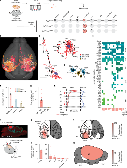
ACA, anterior cingulate area (d, dorsal); AIp, agranular insular area, posterior; APr, area prostriata; Aud, auditory cortical area (d, dorsal; p, primary; po, posterior; v, ventral); AuT, auditory and temporal cortical area; BS, brainstem; CB, cerebellum; CLA, claustrum; ECT, ectorhinal area; ENT, entorhinal area (l, lateral; m, medial dorsal); EPd, endopiriform nucleus, dorsal; FrM, frontomotor cortex; HPF, hippocampal formation; HVAs, higher visual areas; Mo, motor cortical area (p, primary; s, secondary); NC, neocortex; OB, olfactory bulb; Olf, olfactory areas; PAR, parasubiculum; PERl, perirhinal area; PIR, piriform area; POST, postsubiculum; PRE, presubiculum; RSP, retrosplenial cortical area (agl, lateral agranular; d, dorsal; v, ventral); RSPagl, retrosplenial area, lateral agranular; RSPd, retrosplenial area, dorsal; S1, primary somatosensory cortex; SS, somatosensory cortical area (bfd, barrel field; ll, lower limb; m, mouth; p, primary; ul, upper limb; tr, trunk; un, unassigned; s, supplemental); StP, striatum–pallidum; SUB, subiculum; TEa, temporal association area; V1, primary visual cortex; VIS, visual area (a, anterior; al, anterolateral; am, anteromedial; l, lateral; li, laterointermediate; p, primary; pl, posterolateral; pm, posteromedial; por, postrhinal; rl, rostrolateral); VISC, visceral area.

Surgical procedures

Mice were anaesthetized with isoflurane (5% by volume for induction and 1–2% for maintenance), placed on a stereotaxic frame and kept warm with a closed-loop heating pad. For pain management, mice were given intraperitoneal (i.p.) meloxicam at 2.5 mg kg⁻¹ and local lidocaine on the scalp before skin incision. The following coordinates are distance (in mm) from bregma and dorsoventral (DV) values refer to brain surface.

For viral injections, we minimized brain damage by performing burr holes, keeping a thin layer of the bone intact where the glass micropipettes could penetrate.

For wide-labelling morphological reconstructions, 50 nl viral vector was injected into a burr hole split across two levels (DV −0.25 and DV −0.55) at anteroposterior (AP) −3.3, mediolateral (ML) ±2.7 to target primary visual cortex (V1); or at AP −1, ML ±3 to target primary somatosensory cortex (S1).

For silicon probe-coupled optogenetic experiments, four burr holes were drilled centred over V1 (AP −3.3, ML ±2.7) spaced around 1 mm apart, and positioned to avoid blood vessels visible through the skull. Virus (500 nl) was injected into each burr hole split across two levels (DV −0.25 and DV −0.55) for a total of 2 µl virus.

For calcium imaging-related surgeries, mice were also administered dexamethasone at 4 mg kg⁻¹ 1 h before craniotomy. A 3-mm craniotomy was made over V1, and, if applicable, virus was injected into the centre of this craniotomy while the brain was kept moist with hydrated gelatin surgical foam. Then a cranial window was placed over the opening and sealed to the skull with cyanoacrylate glue. For imaging Sst-Chodl cells in superficial layers, the cranial window consisted of a stack of three coverslips: two 3-mm #1 glass coverslips (Warner Instruments) attached with Norland Optical Adhesive 71 to a 5-mm glass coverslip, allowing the 3-mm glass to sit against the dura to discourage bone regrowth⁵⁴. For imaging Sst-Chodl cells in deep layers, durotomy was performed before implantation of a 1.5-mm microprism (A1 coated, 4531-0023, Tower Optical) attached with Norland Optical Adhesive to a single 3-mm glass coverslip.

For pan-neocortex viral delivery, 22 burr holes were split bilaterally and 400 nl of viral vectors was injected at the following coordinates: AP +1, ML ±3, DV −1; AP +1, ML ±1.8, DV −0.4; AP −0.5, ML ±3.8, DV −1.5; AP −0.5, ML ±2.6, DV −0.4; AP −2, ML ±4, DV −1.2; AP −2, ML ±3.2, DV −0.3; AP −2, ML ±1.2, DV −0.3; AP −3.5, ML ±3.5, DV −0.3; and AP −3.5, ML ±2, DV −0.3; and 800 nl of viral vectors was injected at the following coordinates: AP 2.5, ML ±1.2, DV −1; and AP 0, ML ±1, DV −0.5.

For rabies tracing experiments, a total volume of 500 nl of the helper mixture (2:1 ratio optimized glycoprotein over avian tumour virus receptor A (TVA)) split across two levels (DV −0.25 and DV −0.55) was injected into a single burr hole at AP −3.3, ML ±2.7. After a minimum of four weeks to allow robust expression of the helper constructs, rabies vector was delivered as a single injection of 150 nl at the same AP–ML coordinates and DV −0.4. Mice were perfused 10 days after rabies delivery to capture the full extent of monosynaptic retrograde labelling while minimizing cytotoxicity.

For calcium imaging and whole-neocortex chemogenetic experiments, a separate burr hole was made in contralateral above V1 and a made-in-house microwire array connected to a 16-channel omnetic (A79038-001, Omnetics Connector), used for measuring LFPs, was inserted. The LFP wires consisted of five to eight tungsten wires, 50 µm in diameter, spanning from the middle layers of V1 area into cornu ammonis area 1 (CA1). For calcium imaging combined with flexible 32-channel probes (tetrode configuration, NeuralThread⁵⁵), an electrode attached to a stainless steel pole with adhesive polyethylene glycol was inserted perpendicular to the brain at the border of the craniotomy. Then, the polyethylene glycol was dissolved by applying saline continuously for 10 min on top of the pole to ensure its disengagement from the electrode. After pulling the pole straight up out of the brain, the cranial window was positioned above the electrode.

For multi-site LFP and optogenetic experiments, eight burr holes were made at the following coordinates: anterior: AP+ 1.35, ML −2.8 and AP +0.7, ML −1.2; distal: AP +0.05, ML −2.8 and AP −0.6, ML −1.2; medial: AP −1.25, ML −2.8 and AP −1.9, ML −1.2; proximal: −2.55, ML −2.8 and −3.2, ML −1.2. A made-in-house microwire array consisting of eight tungsten wires of 200 µm in diameter, were aligned to the mouse skull, connected to a 16-channel omnetic and inserted in the surface of the brain. Virus (500 nl) was injected ipsilateral of the multi-LFPs at AP −2.7, ML −2.7 split across two levels (DV −0.25 and DV −0.55), and a fibre-optic cannulae of 400-µm diameter and 6-mm length was positioned at the entrance of the burr hole.

Injections were performed using a Nanoject III system at a rate of 1–2 nl s⁻¹ through glass micropipettes that were pulled and then ground to bevel with 40-µm diameter using a Naragishe diamond wheel. For LFPs and flexible probes, a tungsten ground wire of 200 µm diameter attached to a gold pin was inserted into the cerebellum, and a headpost was implanted as previously described⁵⁶.

All implants were secured to the skull using Optibond or Super-Bond followed by dental cement. When Nos1^creER+/− mice were used, tamoxifen (Thermo Fisher Scientific) was administered at least 2 weeks after surgery. A stock solution of 20 mg ml⁻¹ tamoxifen in corn oil was injected i.p. at 0.1 mg tamoxifen per g body weight for 5 consecutive days. Mice were left for a minimum of 4 weeks for CreER-mediated recombination before experimental use.

The following AAV viral vectors were used in this study at concentrations of 10¹²–10¹³ vg ml^–1 (written in the format AAV vector, serotype, source):

• Ef1a-CreOn/FlpOn-oScarlet, 8, provided by the laboratory of K.D.

• Ef1a-CreOn/FlpOn-GCaMP6m, 8, provided by the laboratory of K.D.

• hSyn-CreOn/FlpOn-ChR2-EYFP, DJ, UNC Vector Core

• EF1a-fDIO-mCherry, 5, Addgene (114471)

• nEF-CreOn/FlpOn-hM3Dq-mCherry, 8, provided by the laboratory of K.D.

• nEF-CreOn/FlpOn-TVA-mCherry WPRE, 8, Gene Vector and Virus Core (GVVC; AAV-197), Wu Tsai Neurosciences Institute, Stanford University

• Ef1a-CreOn/FlpOn-oG WPRE, 8, GVVC (AAV-198)

• EnvA-DG-Rabies-EGFP, not applicable (N/A), Salk Vector Core

• iSSTe4-ChR2-mCherry, 1, provided by the laboratory of G. Fishell⁵⁷

Immunohistochemistry

Mice were perfused transcardially with ice-cold 4% paraformaldehyde (PFA) and brains were dissected and post-fixed in 4% PFA for 1 h at 4 °C. After sucrose cryoprotection, brains were embedded in OCT, cryosectioned at 20 µm and adhered to glass slides. For staining, sections were incubated in a blocking solution containing 1.5% donkey serum, 1% Triton-x-100 for 1 h at room temperature. Primary antibodies were applied overnight at 4 °C, followed by washes and 1-h incubation in secondary antibodies. Tissue sections were mounted in Prolong Gold with DAPI (Thermo Fisher Scientific) and imaged on a Zeiss Axioscan slide scanner and a Zeiss LSM 880 confocal microscope for high-resolution imaging.

The following antibodies were used in this study (written in the format antigen target, concentration, vendor, product number):

• Somatostatin (SST), 1:250, Millipore, MAB354

• Somatostatin-14 (SST), 1:1,000, Peninsula, T-4103

• Parvalbumin (PV), 1:1,000, SYSY, 195004

• Vasoactive intestinal peptide (VIP), 1:250, SYSY, 443005

• Neuronal nitric oxide synthase (nNOS), 1:500, Abcam, ab1376

• CTIP2, 1:500, Abcam, ab18465

• SATB2, 1:500, SYSY, 327004

• GFP (reactive against EYFP), 1:500, Invitrogen, A-111222

• RFP (reactive against mCherry), 1:250, Chromotek, 5f8

Tissue clearing and light-sheet imaging

Mice were prepared as described above for morphological reconstruction. Mice were then transcardially perfused with ice-cold 1× PBS followed by 4% PFA. Brains were dissected and post-fixed in 4% PFA at 4 °C for 24 h. Brains were processed with SHIELD reagents (LifeCanvas Technologies) before beginning active tissue clearing using the SmartBatch+ system (LifeCanvas Technologies) using manufacturer protocols. Tissues were refractive index-matched using EasyIndex (LifeCanvas Technologies) and imaged on a SmartSPIM light-sheet microscope (LifeCanvas Technologies) with a 3.9× magnification objective (NA: 0.2, manufactured by Thorlabs and modified by LifeCanvas Technologies). Data were aligned to the Allen Mouse Brain Common Coordination Framework (CCF) using NeuroInfo (MBF Bioscience).

Whole-brain sparse labelling and reconstructions

Whole-neuron morphology data were generated using HortaCloud⁵⁸, an open-source, cloud-based neuron reconstruction platform. Morphological reconstructions were performed on gene-defined, sparsely labelled individual neurons imaged across the entire mouse brain using two-photon fluorescent micro-optical sectioning tomography (fMOST)^59,60. For each neuron, the full local and long-range axonal arbor and dendritic trees were manually identified and traced by an experienced annotator. A second independent annotator then proofread the initial reconstruction and added missed branches and removed incorrectly identified segments. All branch points and terminal endings were verified to ensure complete reconstruction of each neurite. Any discrepancies between annotators were resolved by consensus before the reconstructed cell was deemed final.

Slice electrophysiology and oIPSCs

Acute coronal slices of the neocortex were prepared from adult Sst^flp+/+;Nos1^creER+/− mice of either sex injected with AAV-CreOn/FlpOn-ChR2-EYFP (1 µl split across two depths) (DV −0.25 and DV −0.55) at AP −3.3, ML ±2.7, 5–8 weeks before recording. Mice were anaesthetized with isoflurane and transcardially perfused with ice-cold NMDG-based cutting solution containing (in mM) 92 NMDG, 2.5 KCl, 1.25 NaH₂PO₄, 30 NaHCO₃, 20 HEPES, 25 glucose, 2 thiourea, 5 sodium ascorbate, 3 sodium pyruvate, 0.5 CaCl₂·2H₂O and 10 MgSO₄·7 H₂O, adjusted to pH 7.3–7.4 with 5 M hydrochloric acid. The brain was dissected rapidly and sectioned at 250–260 µm with a vibratome (VT1200S, Leica), and allowed to recover in the same solution for 5-10 min at 34 °C before transfer to warm artificial cerebrospinal fluid (ACSF) containing (in mM) 120 NaCl, 25 NaHCO₃, 1.25 NaH₂PO₄, 3 KCl, 1 MgCl₂, 1.5 CaCl₂, 11 glucose, 3 sodium pyruvate and 1 sodium ascorbate equilibrated with O₂ and 5% CO₂. Slices were incubated for another 30 min and then kept at room temperature until recording for up to 8 h. For a subset of experiments, we used a sucrose-based cutting solution containing (in mM) 90 sucrose, 60 NaCl, 5 MgCl₂, 2.75 KCl, 1.25 NaH₂PO₄, 1.1 CaCl₂, 9 glucose, 26.5 NaHCO₃, 3 sodium pyruvate, 1 sodium ascorbate, equilibrated with 95% O₂ and 5% CO₂. Slices were transferred directly to warm ACSF after cutting under these conditions.

We verified the presence of ChR2-EYFP-expressing fibres in each slice at various distances from the injection site before recording. Putative postsynaptic neurons were recorded across all cortical layers and at various distances from the injection site at near-physiological temperature (around 32 °C) with an internal solution containing (in mM) 15 CsCl, 120 caesium gluconate, 8 NaCl, 10 HEPES, 2 MgATP, 0.3 NaGTP, 0.2 EGTA and 2 mg ml⁻¹ biocytin for post-hoc anatomical analysis (pH adjusted to 7.2 with CsOH; osmolarity adjusted to 290 mOsm). The chloride reversal potential was around −44 mV, and GABAergic currents were recorded at a holding potential of 0 mV. Visually guided whole-cell recordings were obtained with patch pipettes of around 3-MΩ resistance pulled from borosilicate capillary glass (BF150-86-10, Sutter Instrument). Electrophysiology data were acquired using a Sutter dPATCH amplifier (Sutter Instrument), digitized at 10 kHz and filtered at 5 kHz. oIPSCs were evoked with 0.5-ms whole-field pulses of blue light (CoolLED) at a frequency of 0.2 Hz. To isolate inhibitory currents in voltage-clamp, the following receptor antagonists were added to the bath solution: 2 µM (R)-CPP, 5  µM NBQX and 1.5 µM CGP to block NMDA, AMPA and GABA_B receptors, respectively. To confirm GABAergic identity, oIPSCs were blocked with 50 µM gabazine SR95531 in some experiments. To confirm that oIPSCs were monosynaptic, 0.5 µM TTX and 100 µM 4-AP were included in the bath solution in a subset of experiments. All drugs were purchased from Abcam, Tocris or HelloBio. After recording, the patch pipette was withdrawn slowly to allow resealing of the membrane and slices were fixed in 4% PFA overnight. Biocytin-filled neurons were labelled with streptavidin–Alexa 647 using standard protocols. Confocal z-stacks of streptavidin-labelled neurons and EYFP⁺ Sst-Chodl fibres were taken on a Zeiss LSM 880 microscope at 1–2-µm increments. z-stacks were processed in ImageJ and their positions in the cortex were recorded.

Habituation and head restraint

Mice were briefly habituated to handling for several days before surgery. Mice were allowed to recover for 2 days before continuing habituation to handling. After a minimum of 1 week after implantation, mice were gradually exposed to the head-fixation apparatus (https://github.com/janelia-experimental-technology/Rodent-Belt-Treadmill), which consists of a low-friction rodent-driven belt treadmill. The head-fixation duration was gradually increased over 2 weeks until the mice were comfortable with multi-hour head fixation sessions.

To promote sleep while head-fixed, mice were given multiple habituation sessions on the recording rig before data collection. We ensured that the treadmill was oriented horizontally with no slope, with the distance between the head fixation level and the treadmill properly adjusted. The set-up was cleaned thoroughly to minimize odours from other mice, and a radiant heat lamp was provided.

Videography

Videos of mice were acquired using FlyCapture 2 software, at 30 Hz using Blackfly machine-vision ethernet-enabled cameras (FLIR) equipped with a Basler lens (model c125-1620-5m) for head-fixed experiments and a Computar lens (TG4Z2813FCS-IR 0.33-Inch) for freely moving experiments. Rigs were illuminated with infrared LED arrays, similar to methods described previously⁶¹. The camera was configured to send transistor–transistor logic (TTL) pulses to synchronize videography with other data streams.

In vivo two-photon calcium imaging

GCaMP was expressed either using an AAV-CreOn/FlpOn-GCaMP6m viral vector or through transgenic expression in the Ai210 mouse line (a Cre- and Flp-dependent GCaMP7f). No substantial differences were observed between the two approaches. Mice were imaged on a custom Bergamo two-photon microscope coupled to a Ti:Sapphire laser (Mira 700, Coherent). Emitted light was collected through a 10× 0.5-NA long-working-distance objective (TL10X-2P, Thorlabs). Images were typically acquired with ThorImage software at 1.4 frames per second with a resolution of 512 × 512 pixels and, for experiments coupled with flexible probes, at 14.6 frames per second with a resolution of 128 × 128 pixels. For microprism data, cell positions were estimated from the distance of the soma relative to the visible-damage layer produced by microprism insertion, which was used as a reference for the cortical surface (estimation relative to the Allen Brain Atlas). Data streams were synchronized using TTL pulses collected on an RHD USB interface board (Intan Technologies) at 20 kHz. Before imaging, novel objects were placed in the mouse’s home cage, one per hour for up to 4 hours, to promote exploration and subsequently facilitate sleep during imaging.

Acute in vivo electrophysiology and optogenetics

Mice were injected with AAV-CreOn/FlpOn-ChR2-EYFP and implanted with headposts as described above. After viral expression, tamoxifen induction and treadmill habituation, mice were administered dexamethasone (4 mg kg⁻¹, i.p.) 1 h before craniotomy. An approximately 3-mm craniotomy was made over the injection site (V1).

A 64-channel linear silicon probe (H3 probe, Cambridge NeuroTech) physically coupled to a tapered optical fibre was slowly (1 µm s⁻¹, over around 20 min) inserted into V1. The craniotomy was kept moisturized during the recording by placing a small volume of silicon oil on the surface of the brain. State measurements were made as described below. Between recording days, the craniotomy was protected with KWIK-CAST silicon elastomer (World Precision Instruments). Mice were recorded once per day for 3–4 days.

Recordings were split into blocks of around 30-min spontaneous periods (without stimulation) and around 30-minute periods of stimulation. Several types of stimulation were used, including sinusoids (1 Hz, 4 Hz, 10 Hz and 40 Hz), flat pulses and white noise, each delivered for 30 s followed by a 30-s ITI. Blue light was provided by a fibre-coupled LED (MF470F4, Thorlabs). Signals to control LED light intensity were generated using custom-written MATLAB software and delivered to an NI DAQ card (NI-PCIe-6323) to be output to the LED control box (LEDD1B, Thorlabs). No light artefacts were detected in our recordings.

Across more than 700 recorded single units, plus additional multi-units from 10 mice, no optotagged units were found, underscoring the extremely low abundancy of this neuronal population and the difficulty of capturing the cells directly in silicon probe recordings.

Data were acquired using an Intan RHD2000 interface board at 20 kHz.

Multi-LFPs and optogenetics

Mice were injected with AAV-CreOn/FlpOn-ChR2-EYFP and implanted with headposts as described above. Recordings were split into blocks of around 30-min spontaneous periods (without stimulation) and around 30-min periods of stimulation using a 10-Hz sinusoid frequency. Similar to the acute recordings, the stimulation periods consisted of 30 s of blue light followed by a 30-s ITI. The optical and acquisition hardware used was the same as that described above.

Freely moving behavioural assay

Mice were injected with AAV nEF-CreOn/FlpOn-hM3Dq-mCherry or control EF1a-fDIO-mCherry, implanted with LFP wires as described above and single-housed after surgery. Mice were habituated to wired tethering via a 16-channel digital headstage with an accelerometer (Intan Technologies) and connected to a motorized commutator (Doric Lenses or Neurotek). To minimize stress and noise distraction, mice were kept in their home cage in an acoustic foam box for 2 h per day for 3–5 days. Mice were also habituated to receiving systemic saline injections at the beginning of the session for at least 2 days before monitoring their behavioural state. A consistent time of day was used for each mouse during the light (inactive) phase (ZT3–ZT7) or during the dark (active) phase (ZT18), and this was maintained throughout the experiment. No differences in sleep behaviour were detected across specific ZT windows used within the light (inactive) phase, but sessions during the light (inactive) and the dark (active) phase were analysed separately.

After habituation, mice received i.p. injections of either vehicle (saline) or CNO (HelloBio) at 0.5 mg kg⁻¹. This dose has been shown to have no effect on the sleep of control mice without DREADD treatment^62,63, and we confirmed this in our control experiment (12 sessions from 6 mice during the light phase, Extended Data Fig. 9l–o). The initial treatment was counterbalanced across mice, and the alternative treatment was administered the following day. Thus, each session was paired with its opposite treatment for analysis (vehicle versus CNO or CNO versus vehicle). Mice completed two vehicle and two CNO sessions, and data for each treatment were averaged across the two sessions. To ensure sufficient wakefulness, only mice that remained awake for at least 60% of the time during vehicle sessions were included in the analysis within the light or dark phase. We obtained a total of 28 sessions during the light phase from 14 mice and 12 sessions during the dark phase from 6 mice.

LFP data were acquired at 1,250 Hz using an Intan RHD2000 interface board.

Behavioural state scoring

Behavioural state was divided on the basis of a combination of the acquired state measurements. First, to score sleep states we used previously published and validated methods implemented in the Buzcode toolbox from the Buzsaki lab^64,65. In brief, this method provides automatic state scoring by distinguishing SWS from wake using the slope of the power spectrum (a large slope occurs during high delta periods of sleep). REM sleep is identified as periods of high theta/delta ratio with low EMG. The automatic scoring is then visualized and manually refined by experts. For optogenetic and chemogenetic experiments, state was scored using LFPs that were recorded outside the neocortex, in the hippocampus, to provide an accurate measure of state. All sleep scoring was done blinded to stimulation conditions (optogenetic or chemogenetic).

The remaining periods of wakefulness were then divided into movement and quiet wake (QW) states. In head-fixed recordings, movement intervals were defined as periods of 5 s or longer in which facial motion energy (extracted using Facemap, binned at 1 s) exceeded the 90th percentile of the session’s distribution. QW was defined as the remaining wake intervals, with a minimum duration of 5 s. A similar procedure was applied in freely moving experiments, but accelerometer signals were used instead of the facial motion to classify movement and QW states. We noted that head-fixed mice exhibited substantially longer QW periods than did freely moving mice, and we confirm, consistent with previous reports, that head-fixed mice sleep with their eyes open, and exhibit typical LFP signatures (high delta power during SWS and high theta/delta ratio during REM)⁶⁶. Although episodes of QW, REM and SWS in head-fixed mice might differ in meaningful ways from those recorded in freely sleeping mice, we used the same state terminology across head-fixed and freely moving experiments for consistency.

Data analysis

Data were analysed using open-source software packages and custom-written MATLAB (2018b–2023b) and Python code.

Whole-neuron morphology projection matrix

SWC files were merged and resampled so that spacing between nodes was uniform. Merged files were registered to the average mouse brain template of the Allen Mouse Brain CCF (v.3)⁶⁷. CCF-registered reconstructions were translated so that all somas were positioned on the left hemisphere. To generate a projection matrix, we used two strategies: one included all axons present in an area (Fig. 1, Supplementary Table 1 and Extended Data Fig. 1), and the other required that a targeted structure contain at least one branch tip and one node (Supplementary Table 2). All projections were ipsilateral, and targeted structures are reported only for the ipsilateral hemisphere.

Whole-brain fibre density and rabies

Mice were cryosectioned as described above, with uniform sampling throughout the entire brain. Imaged brain sections were aligned to the Allen Mouse Brain CCF using NeuroInfo (MBF Bioscience), with the BrainMaker workflow. Labelled neuronal arbor in aligned tissue was then reconstructed within single sections using Neurolucida 360 (MBF Bioscience). Density measurements for individual areas were made by calculating the total path length of reconstructed arbor within that area divided by the volume of the area (the two-dimensional area within section multiplied by the section thickness). The coordinates of each identified rabies-positive neuron were compiled to yield a complete whole-brain map for each mouse. To account for variability in labelling efficiency between mice, data from each brain were normalized to the total number of rabies-positive cells identified in that mouse. These normalized values were then used for quantification of layer distributions, regional localization and subregional visual cortex analyses.

Ex vivo patch-clamp recordings

Electrophysiology data were analysed using SutterPatch v.2.4 (written in IgorPro, Wavemetrics) and AxoGraph v.1.7.6. oIPSCs were aligned to the light stimulus and 20–60 traces were averaged to calculate oIPSC amplitude and latency. Amplitude was measured as the maximum positive peak of the baseline-subtracted oIPSC, and latency was calculated as the time between the light stimulus and crossing a 2 s.d. threshold of the oIPSC from baseline.

Extraction of calcium activity

Acquired images were processed using Suite2p (ref. ⁶⁸) to extract regions of interest and fluorescence traces. ΔF/F₀ values were computed by normalizing fluorescence to a moving 10th percentile within 10-min windows as the baseline (F₀). Deconvolved calcium signals were obtained from Suite2p, and, owing to their higher temporal resolution, were used to examine the temporal relationships between calcium activity, delta power, state transition and DOWN states. To investigate state transition, calcium activity was evaluated only during states lasting a minimum of 10 s. The latency of calcium activation during SWS was defined as the earliest time point at which the deconvolved calcium signal exceeded 2 s.d. above baseline activity. When measuring calcium activity around DOWN states, calcium traces were corrected by subtracting chance-level calcium activity generated by circularly shifting the calcium signal (circshift in Matlab) 100 times within the 1-s window around the onset of DOWN states.

Arousal score

Arousal score (Fig. 2b) was calculated using the pca function in MATLAB. It corresponds to the time-varying score for the first principal component of the measured state metrics. Principal component loadings were calculated for each individual recording to provide robustness against measurement error for any singular state metric.

Classification of low-arousal- and high-arousal-correlated cells

Cell types were determined on the basis of the correlation of ΔF/F traces with state metrics. k-means clustering (n = 2) was performed on these correlation coefficients. Separately, we calculated the correlation coefficient of the ΔF/F signal with the arousal score. Cells with negative correlation coefficients (low-arousal-correlated cells) overlapped completely with the k-means low-arousal cluster.

High- versus low-Sst-Chodl cell activity epochs

ΔF/F traces were averaged within each recording and then z-scored. High-activity epochs were defined as periods in which activity was more than 2 s.d. from the mean, and low-activity epochs were defined as those in which activity was less than 0.5 s.d.

Single units and LFP extraction

Single units were isolated using Kilosort2 (ref. ⁶⁹). Figures contain data from both broad-spiking and narrow-spiking units, because no differences were found between these groups. LFP signals were collected from the microwire array or from silicon probes and were downsampled to 1,250 Hz. EMG signals were obtained by band-pass-filtering the raw signal (more than 200 Hz) followed by a Hilbert transform.

Calculation of power spectra

Power spectra were calculated using a wavelet-based spectrogram method (Morlet wavelets, five-cycle width). These wavelets were generated for 100 log-spaced frequencies from 1 Hz to 128 Hz. For freely moving optogenetic experiments, changes in power spectra were assessed by comparing the 30-s stimulation periods to the 30-s ITIs. To investigate changes in power spectra across the neocortex as a function of distance from the injection site, we selected, at each distance (proximal to anterior), the channel that showed the largest delta band power increase. This approach was implemented to minimize the confounding effects of asymmetrical projections in which Sst-Chodl fibres might be absent on one side but present on the other at a single distance, given the substantial variation in individual projection patterns (see Fig. 1).

Determination of cortical depth

As shown previously, high-frequency power (more than 500 Hz) peaks in mid-layer 5 (ref. ⁷⁰). We interpolated between this layer 5 channel and the first channel outside of the brain (1.3 mm probe inserted 1.2 mm into the brain), assuming the remaining distance, without the mechanical deformation of the brain caused by insertion of the probe, to be 700 µm. With these interpolated pseudo-depths, we then defined layer boundaries at 100, 300, 450, 650 and 900 µm.

Spiking synchrony

The cross-correlation was calculated for each unit pair using default parameters of the CCG.m function from the Buzcode package. The spike times of these units were shuffled, and the cross-correlation was recalculated 100 times to estimate a chance level. The real cross-correlation was then normalized by this chance level to quantify spiking co-activation.

Phase locking

The Fourier spectrum of the LFP was calculated for each spike from each unit using the ft_spiketriggeredspectrum function from the FieldTrip toolbox. The circular mean of the phase values at each frequency was calculated as the phase locking value. Although this measure is sensitive to spike count, with higher spikes leading to higher phase locking values, we do not see this as an issue, because stimulation leads to slightly lower firing rates compared with baseline.

DOWN state detection

DOWN states were detected using a previously published method²⁷. In brief, the method detects a confluence of a large positive deflection in LFP, a drop in gamma-band power and a sharp drop in the multi-unit firing rate.

Linear regression model

Deconvolved calcium signals were used to predict the z-scored delta amplitude after constructing a time-lagged design matrix spanning a 20-s temporal window, sampled every 0.2 s. The kernel was centred on the present time point, allowing both past and future lags to contribute to the prediction. Ordinary least-squares regression was fitted in a fivefold cross-validation scheme, and model performance was quantified by the cross-validated coefficient of determination (R²). The resulting regression weights were averaged across folds to obtain a mean temporal kernel describing the influence of calcium activity at different lags on the predicted delta signal.

Mouse tracking

Cage position and mouse nest area were delimited manually using a compilation of frames extracted every 10 min from each video. Mouse position was detected from the body centroid of the mouse using the DeepLabCut open-source system⁷¹. The distance moved by the mouse was extracted according to the registered position of the cage. The duration spent in the nest was estimated by calculating the time that the mouse was present in the nest according to the total duration of the experiment.

Allen Brain Observatory data analysis

Sst-expressing cell state correlation data were retrieved using the Allen SDK and querying the database for all experiments performed with Sst^cre and Cre-dependent GCaMP mice. Pearson’s correlations were calculated between activity traces and state metrics after binning both signals into 3-s windows. Data on the proportions of Sst-Chodl cells within the Sst population were retrieved from a previously published dataset⁸ from the web-based Brain Knowledge Platform (https://knowledge.brain-map.org/data).

Analysis of previously published data

Data were retrieved from https://doi.org/10.6084/m9.figshare.19448531 (ref. ²⁹), and analysed from spontaneous recordings without visual stimulation.

The following software packages were used to analyse the data presented in this paper (written in the format package name, URL, publication):

• AllenSDK, https://github.com/AllenInstitute/AllenSDK, N/A

• Buzcode, https://github.com/buzsakilab/buzcode, N/A

• Facemap, https://github.com/MouseLand/facemap, ref. ⁷²

• Suite2p, https://github.com/MouseLand/suite2p, ref. ⁶⁸

• Kilosort2, https://github.com/MouseLand/Kilosort, ref. ⁶⁹

• FieldTrip, https://www.fieldtriptoolbox.org/, ref. ⁷³

• DeepLabCut, https://github.com/DeepLabCut/DeepLabCut, ref. ⁷¹

• Phy v.2.0 beta, https://github.com/cortex-lab/phy, N/A

• SutterPatch v.2.4, https://www.sutter.com/amplifiers/sutterpatch, N/A

• AxoGraph v.1.7.6, https://axograph.com/, N/A

• HortaCloud, https://doi.org/10.1101/2025.03.13.642887, N/A

• MBF Bioscience, https://www.mbfbioscience.com, N/A

• MATLAB v.2018b–2023b, https://www.mathworks.com, N/A

Statistical analysis

MATLAB (MathWorks, v.2018b–2023b) was used for statistical analysis. No power calculations were used to predetermine sample sizes or to formally assess normality. The sample size (mice, sessions, cells and units) is consistent with similar studies in the field^21,22,39 and reflects the technical complexity of the manipulations and recordings, and their yield. Chemogenetic experimental mice were randomly assigned to receive CNO or vehicle injection in the first session. Other experimental conditions were defined by recording site, genetic targeting or stimulation protocols independent of the group assignment. Comparisons were performed using two-tailed parametric t-test or one-way, two-way (anova1) or repeated-measures ANOVA, with post-hoc Bonferroni corrections for multiple comparisons (unless stated otherwise). Differences in proportions were assessed using Chi-squared tests (chi2cdf). For optogenetic experiments (linear probes, multi-LFPs and patch clamp) and comparison of SWS duration between light and dark sessions, a linear mixed-effects model was implemented in MATLAB (fitlme) and the model significance was assessed by ANOVA, which tests for the contribution of each fixed factor and their interaction while accounting for unequal sample sizes. Values and statistical tests used are reported in the text and data are represented as mean ± s.e.m. unless stated otherwise. Significance was set with α = 0.05 and is represented on graphs as *P < 0.05, **P < 0.01 and ***P < 0.001.

Reporting summary

Further information on research design is available in the Nature Portfolio Reporting Summary linked to this article.