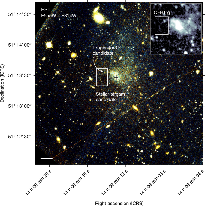
Data

The HST Advanced Camera for Surveys (ACS) images use the Wide Field Channel (WFC) in the F555W and F814W filters, have an angular resolution of 0.1″ and reach exposure times of 2,406 s and 2,439 s, respectively. The observations were carried out in September 2022 under HST programme ID 16890 (ref. ⁵²) and the resulting images of UGC 9050-Dw1 were presented in ref. ¹⁷. The images have been calibrated through the standard HST CALACS pipeline and are available on the STScI/MAST archive.

Thank you for reading this post, don't forget to subscribe!

CFHT has observed the same region of the sky using MegaCam as part of its Legacy Survey in 2005 and UGC 9050-Dw1 was first identified and selected in a semi-automated search for diffuse dwarfs¹⁹. The area containing UGC 9050-Dw1 is visible in both the W3-1-3 and W3-2-3 fields of the survey, which contains bands u, g, r, i and z, so a total of ten CFHT images are available. Because of the signal-to-noise levels, we are not able to confidently identify the stream-like feature in the u-band or z-band images. Integration times, observation depth and seeing for the CFHT data are published in ref. ⁵³. The CFHT data, which have been calibrated through the MegaPipe pipeline, are available through the Canadian Astronomy Data Centre.

For visual purposes, we have smoothed the HST and CFHT images using a Gaussian kernel (with σ = 3 and 1.5 pixels, respectively) and we plot the area of interest in all available bands in Extended Data Fig. 1. All data analysis is performed on unsmoothed data.

Data analysis

The feature was initially detected by eye, but when we apply the rolling Hough transform⁵⁴ with a range of (hyper)parameters, the code consistently returns both the location and curvature of the stream candidate. We use this as a validation of the initial by-eye detection.

In Extended Data Fig. 2 (left), we rotate the images into a coordinate frame aligned with the stream, in which (ϕ₁, ϕ₂) represents stream longitude and latitude^55,56. We draw masks around the stream by following a polynomial fit to points selected manually in the F814W image, creating a curved shape with constant width, excluding the GC candidate. We duplicate these on both sides to mask the background areas. To measure the width, we sample slices perpendicular to the track curvature in steps of pixel size along this fit. We collapse the resulting area along the fitted track, calculating the mean brightness of the stream candidate and its surrounding areas. The right panels of Extended Data Fig. 2 depict the perpendicular brightness profile, consisting of the average brightnesses measured parallel to the curved stream track. This is done in six segments to check for any single dominating contaminant. We fit a Gaussian with a linear offset to the perpendicular brightness profile for each segment, as well as the whole stream. This way of sampling the surrounding area causes the inner part of the curve to be oversampled compared with the outer curve and thus, by construction, it has a lower error and dominates the fit. We therefore use the average of all standard deviations as uniform errors. The standard deviation of the Gaussian provides an estimate of the width of the stream, with uncertainties on the fitted parameter. Because σ describes the deviation from the mean, μ, the total width is twice σ. We denote this width, measured from μ − σ to μ + σ, as w_±σ. The width that includes 95% of the Gaussian area, corresponding to 2σ from the mean, we call w_±2σ. The physical width is affected by the instrument point spread function (PSF), which we account for by subtracting the observational dispersion in quadrature. We use the full width at half maximum for HST of 0.1″.

The seeing of the CFHT observation (0.88″) is comparable with the width of the feature in the CFHT images (w_±σ = 1.1″). Therefore, we use the HST width in subsequent analysis.

There is a brighter object located next to the track at around ϕ₁ = −4, which increases the measured width. If we only use the track up to that point, it yields a width of w_±σ = 52 pc instead. On the other hand, the faintness of the object means that we might only be sensitive to the brightest central part of our stream candidate, which would lead to an underestimated width. In Extended Data Fig. 6, we illustrate that the simulated GC streams show up with similar apparent width when injected into the data.

To quantify the prominence of the stream candidate, we sum the counts in the on-stream mask and in the off-stream background masks. We subtract the mean background from the signal and compare this with the standard deviation of the backgrounds: \((Keep following us for the latest insights._For more tech updates, stay tuned to our blog.-\,{\overline{f}}_{{\rm{background}}})/{\sigma }_{{\rm{background}}}\).

The Gaussian fit used in the width measurement also gives a signal-to-noise ratio when we compare the amplitude to its fit uncertainty, \(A/\sqrt{{\sigma }_{A}}\). This uncertainty takes into account the error on the means, which were included in the fit. Neither prominence estimate includes the GC candidate; they are based only on light from the stream candidate.

The statistical significance contains three main components: the probability that it is a stream, the probability that we would find it and, given that the first two statements are true, the statistical significance of the signal in the data. What we quote as a significance is only the last of these.

To compare the colours of the stream and cluster candidates to other GC candidates in the host UDG, we sum their brightness in each of the two available HST filters. The stream area is defined as a curved shape with the constant width found above (w_±2σ = 16.8 pixels = 143.7 pc) around a polynomial fitted to an array of manually selected points along the track. The cluster is contained in a circular mask 20 pixels (170.6 pc) wide, following a photometric growth-curve analysis similar to, for example, ref. ⁵⁷ to find an aperture radius that includes most of the light. We make sure that the masks of the stream and progenitor do not overlap. Both masks are illustrated in Extended Data Fig. 3 with blue and purple outlines, respectively. All magnitudes are in the Vega system and we correct for galactic extinction using values from ref. ⁵⁸ as calculated through the NASA/IPAC Extragalactic Database (NED) extinction calculator.

For accurate colour measurements, we need to subtract the background of a nearby approximately empty equal area (see, for example, ref. ⁵⁹). Owing to the complex morphology of UGC 9050-Dw1, the choice of this area is not obvious and the resulting colour is greatly affected by the choice. We therefore use the average of several areas distributed on both sides of the stream candidate (illustrated in Extended Data Fig. 3). The errors on the colour values reflect the spread resulting from using either of the background areas on its own, as well as the error on the brightness in each band, which is measured by the standard deviation of pixel values.

The ACS pixel scale of 0.05″ per pixel corresponds to 8.53 pc at this distance. This is comparable with the size expected for GCs (a few pc)⁶⁰ and ref. ¹⁷ therefore treats the GC candidates as point sources. For a partially disrupted cluster, however, we expect a larger physical extent and, by definition, a stream will not resemble a point source. We therefore treat both objects as extended sources, using areas illustrated in Extended Data Fig. 3 as their extent. Our GC candidate is not included in the final GC candidate sample of ref. ¹⁷ and inspection of their selection criteria reveals that it is discarded on the basis of roundness, sharpness and/or magnitude uncertainty. A tidally disrupting GC would be both elongated and more diffuse than the undisturbed clusters, which explains the deviation from all three criteria.

We integrate the light over the areas illustrated in Extended Data Fig. 3 to measure the surface brightness of the stream candidate. This yields a surface brightness of 27.0 ± 0.1 and 26.1 ± 0.1 mag arcsec⁻² in the F555W and F814W filters, respectively, after subtracting the background.

To explore the possible stellar populations in the stream, we use a grid of isochrones with varying age and metallicity. We sample stars from a simple initial mass function (IMF) following \(\frac{{\rm{d}}N}{{\rm{d}}m}\propto {m}^{-0.5}\) (ref. ⁶¹) and truncated on the basis of the mass range of survived stars in each of the isochrones. We extract brightnesses from the interpolated isochrone tracks, generated for HST and CFHT filters through the colour–magnitude diagram input form⁶² using the PARSEC version 1.2S evolutionary model⁶³. We distribute these stars across the area of the stream in the data, including the presumed hidden arm, and we calculate their surface brightness. We decrease the population size until there is only one isochrone that gives a surface brightness comparable with that in the HST data. This population is just visible with the brightest isochrone in our suite and we use its total mass as a lower bound on the possible size of a stream with this surface area producing the observed brightness.

We find that an initial progenitor mass as low as M_⋆,tot = 1.65 × 10⁵ M_⊙, with an 8-Gyr-old stellar population with [M/H] = −1.0, can reproduce the observed surface brightness of the present-day stream.

Because we do not know the detailed mass loss history of the GC candidate, to obtain the total mass of the stream and progenitor, we assume that the brightness ratio between the cluster and stream is an appropriate proxy for the mass ratio. Assuming that the two stream arms are identical, this gives a ratio of M_stream/M_total ≈ 0.75, which we use to scale the inferred stream mass to a total progenitor mass.

For the Pal 5-like stream, we use the same methodology to estimate the level of disruption as in ref. ³⁷. We use an isochrone track with age 11.3 Gyr and metallicity of [M/H] = − 1.3. Pal 5 contains 3,000 stars in the DECAM g band between magnitudes 23 and 20 (ref. ⁵⁹), so we sample the IMF until this threshold is reached and use the resulting sample to calculate the surface brightness of the population. We repeat this process for samples of 5, 10 and 20 times the threshold (corresponding to equal multiplications of Pal 5 mass), the last of which yields a surface brightness matching the values from the HST data. This method assumes a mass loss identical to that of Pal 5.

Generative stream models

To generate stream models, we apply the X-Stream sampler⁶, which uses the particle-spray method⁶⁴ implemented in the GPU code streamsculptor⁶⁵. We fix the escape conditions to those of ref. ⁶⁴. These particle-spray simulations are tuned to reproduce more expensive N-body simulations of GC dissolution. Note that our results are dependent on the stream model escape conditions. We generate streams in a halo potential meant to represent the diffuse dwarf with an inner slope, γ, and outer slope, β (see equation (1) in ref. ⁶). We do not include the baryons in our modelling efforts, as these make up a small fraction of mass compared with the estimated mass of the total system (M_* ≈ 10⁷ M_⊙ within the half-light radius)¹⁷. The dark matter halo profile is thus treated as a representation of the entire diffuse dwarf.

We define the coordinate system in which we generate model streams by transforming the candidate GC progenitor position and the centre of UGC 9050-Dw1 from right ascension and declination to a galactocentric rest frame at which UGC 9050-Dw1 is at the origin using astropy⁵⁶ and the distance to UGC 9050-Dw1 of 35.2 Mpc. x and z define the plane of the sky and y is the line-of-sight direction pointing towards the observer. We fix the on-sky position of the progenitor (x, z) in our models.

In this coordinate system, we outline a mask for the observed stream extending to the left of the candidate GC progenitor. To test how the choice of width affects our results, we use two different mask widths to represent the stream. Our fiducial mask width is w_±2σ = 143.7 pc. We also test a mask width of 185 pc corresponding to w_±3σ. We create a grid of control points within the outlined masks to represent the candidate stream. These control points are used as our input for the X-Stream sampler. Note that we only generate control points for the left side of the stream, as we do not confidently observe a right extension of the stream.

From the control points, we generate a kernel density estimation (KDE). For each model stream, the sampler generates a KDE and uses a Kullback–Leibler divergence test^66,67 to measure the difference between the KDE from each generated model stream and the KDE from the input control points (see details in ref. ⁶). The best-fitting model streams are ones that minimize this difference. Note that particle-spray models do not reproduce the detailed density along the stream but that X-Stream relies on control points and includes an inverse density weighing to smooth over features. Streams wider than the data have excess density inconsistent with the control points and X-Stream thereby disfavours wider models.

We draw a bounding box around the stream mask to ensure that we do not penalize our generated model streams if they are longer than the mask nor if they extend to the right of the progenitor. However, the model streams are penalized if they are shorter than the observed stream.

To sample the parameter space and test which orbits, progenitor properties and halo properties can reproduce the present-day observed candidate stream, we use ten free parameters with uniform, flat priors and fix only the progenitor position in the plane of the sky (Extended Data Table 1). We test two different concentrations for the dark matter halo: c = 2 and c = 5 (as motivated from refs. ^3,5). X-Stream uses a nested sampling technique to examine the large parameter space and the sampler outputs the likelihood of each model stream and the likelihood surface, including the 68% and 95% credible regions for all parameters.

Owing to the known degeneracies for the orbital direction of a stellar stream in the plane of the sky (see Figs. 10 and 8 in refs. ^6,33, respectively), we only sample half of the unit sphere in the velocity space. Thus there are islands of solutions for which the model streams move in the opposite direction (that is, opposite leading and trailing arms), which are equally good fits. However, the distance gradient for such solutions remains the same (see Figs. 10 and 9 in refs. ^6,33, respectively). We list all free and fixed parameters for the X-Stream sampler in Extended Data Table 1. See ref. ⁶ for a detailed description of each parameter.

To test which parts of the model streams would be observable in the HST data, we mock-observe three different stellar stream models:

1. 1)

   The lower bound stream: a stream with a progenitor mass of 1.65 × 10⁵ M_⊙ with [M/H] = −1.0 and age 8 Gyr motivated from the surface brightness analysis, which showed that such a stream would be observable in the HST data. We populate this stream with 2.8 × 10⁵ stars corresponding to the simulated population with mass 1.65 × 10⁵ M_⊙ described above.

2. 2)

   The 20× Pal 5-like stream: a stream with a progenitor mass of 2 × 10⁶ M_⊙ with [M/H] = −1.3 and age 11.3 Gyr, which should also be observable in the HST data based on our surface brightness analysis. We populate this stream with 1.17 × 10⁶ stars, again based on the count in our simulated populations.

3. 3)

   A dwarf-like stream: a stream with a progenitor mass of 2 × 10⁷ M_⊙, to mimic a more massive dwarf stream. We use the same stellar population as for the 20× Pal 5-like stream to allow for easy comparison and to reflect that the extra mass is in dark matter.

For each stream model, we sample the IMF up to the stellar mass that survives in the present day and assign each star in the population a magnitude in the F555W and F814W HST bands, interpolated from the chosen isochrone. We sum the distributed flux from all of the stars in the model stream, add Poisson noise and inject the mock stream into the HST image in both bands, convolving the magnitude with an empirical PSF described in ref. ⁶⁸, which uses PSF models from ref. ⁶⁹. We inject each stream in approximately empty areas near the Oyashio stream to facilitate visual comparison.

When calculating the expected surface brightness of the simulated stellar population, we assume that all of the stars are within the mask, which is not the case, especially for the broader dwarf-like stream. To make the dwarf-like stream visible, we multiply the brightness by 5. This illustrates that a stream with a larger area needs a more massive stellar component to achieve the same surface brightness. The images are stacked as in Fig. 1 and shown in Extended Data Fig. 6.

Note that several assumptions go into this analysis, such as the specific isochrones, degree of disruption and the details of the stream modelling. Nonetheless, these mock observations provide a zeroth-order test of which parts of each model stream could be observable in the HST data.