Ethics

The work reported on TwinsUK samples was carried out with informed consent under TwinsUK BioBank ethics, approved by the North West–Liverpool Central Research Ethics Committee (REC reference 19/NW/0187), IRAS ID 258513 and earlier approvals granted to TwinsUK by the St Thomas’ Hospital Research Ethics Committee, later the London–Westminster Research Ethics Committee (REC reference EC04/015). SL samples were obtained from Discovery Life Sciences as discarded medical waste in accordance with IRB protocol DLS-BB050. These were collected as part of standard-of-care testing ordered by the patient’s physician and excess material released for research.

Sperm sample extraction and sequencing

We obtained 15 sperm samples from 13 donors of European ancestry. Eleven individuals donated one sample, and two individuals donated two samples at different ages (AA1-s1 and AA1-s2; AN-s1 and AN-s2), with ages at donation varying between 24 and 74 (Supplementary Table 1). Samples AA2-t1 and AA2-t2 are monozygotic twins. The TwinsUK cohort consists of more than 14,000 volunteers, mostly middle-aged female individuals, who have participated over the past 30 years in a longitudinal cohort study. This has included lifestyle and health questionnaires, biomedical measurements, biological sample collection and the generation of multi-omics profiles (such as genetics, metagenomics and metabolomics), over multiple visits.

For the TwinsUK samples, we obtained high molecular weight (HMW) DNA from bulk sperm samples using the Circulomics Nanobind Tissue Kit (102-302-100) and NEB Monarch HMW DNA Extraction Kit for Cells & Blood (T3050) UHMW with some modifications to account for tighter packing of the sperm genome. We supplemented the lysis solution with 150 mM 1,4-dithiothreitol to disrupt protamine disulfide bonds and extended proteinase K incubation from 30 min to 2 h. The rest of the Circulomics HMW DNA extraction protocol remains unchanged. HMW DNA was sheared to 10–14 kb DNA fragments using Megaruptor 3 system (B06010003) with speed setting 30. CCS sequencing libraries were constructed according to the standard CCS library preparation protocol 1.0 (100-222−300), and the libraries were sequenced using a Sequel IIe and Revio instrument at the Wellcome Sanger Institute with full-resolution base quality scores.

For the SL data, samples were thawed on ice and cells were pelleted in an isotonic sperm wash solution to remove debris and reduce somatic cell contamination. DNA was extracted using the NEB Monarch HMW DNA Extraction Kit for Cells & Blood (T3050) UHMW protocol, with some modifications to the cell lysis step. Specifically, cells were digested at 56 °C for 1 h at 300 rpm with 100 µl Nuclei Prep Buffer, 100 µl Nuclei Lysis Buffer, 10 µl Proteinase K (NEB P8107, 20 mg ml⁻¹), and 10 µl 1 M 1,4-dithiothreitol (GoldBio in dH₂O, final concentration ~50 mM). An additional 20-minute digestion was then performed with 5 µl RNase A (NEB T3018, 20 mg ml⁻¹). The rest of the protocol remained unchanged. HudsonAlpha performed HMW DNA quality control, CCS library preparation, and sequencing on the PacBio Revio sequencing instrument.

Blood sample sequencing data analysis

We obtained raw PacBio CCS sequencing data and assemblies from the Platinum Pedigree dataset. Flow cells containing multiple samples were excluded due to cross-sample contamination caused by demultiplexing errors. Additionally, we excluded the four first-generation samples, as they were derived from cell lines. This resulted in a final dataset of 12 samples.

De novo haplotype-resolved assembly

We used hifiasm³⁰ (v0.19.5-r592, default parameters, HiFi only mode) to construct a haplotype-resolved de novo assembly for each sample. The hifiasm assembler outputs a partially phased assembly graph for the two haplotypes, which we converted into two fasta sequence files per sample.

We scaffolded each haplotype onto the T2T-CHM13 reference genome⁵² with RagTag⁵³ (v2.1.0, with arguments “-u -w –aligner minimap2”). RagTag orients and places contigs along the T2T reference with gaps; we manually expanded the gaps between adjacent contigs to 30,000N to avoid reads mapping across a gap to two contigs, as this may include a phase switch error which will further be falsely interpreted as a CO.

PRDM9 genotyping

We obtained the zinc-finger array sequences from 74 PRDM9 alleles reported previously²⁷ and mapped them to each assembled haplotype of each donor. For each haplotype, we called the PRDM9 allele as the one with the smallest amount of mismatches, insertions or deletions between the allele sequence and the assembly. All the A alleles, B allele and the D allele were a perfect match, whereas we did not find a perfect match to the new PRDM9 allele of AN-s1/2. In addition, we verified that the flanking regions on the two sides of the sequence match the expected sequences as reported²⁷ (up to 2 bp mismatches), and confirmed that PRDM9 allele variations are not due to assembly errors by visually inspecting the assembly around the region.

Read alignment

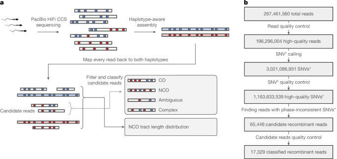
CCS reads with residual adapter sequences were identified with HiFiAdapterFilt⁵⁴ and were excluded from downstream sequence analysis. We used minimap2^55,56 (v2.26-r1175, with arguments “-ax map-hifi –cs=short –eqx –MD”) to map the reads to each haplotype separately. We then filtered each bam file to contain only primary alignments (using the “-F 0×900” flag in samtools view⁵⁷) and with mapping quality MAPQ = 60. We further discarded reads that map to only one of the haplotypes, or that map to different chromosomes. Finally, we discarded reads that map to different strands of the two haplotypes.

Creating candidate recombinant reads

Comparing haplotype alignments

Each alignment of a read to a haplotype effectively partitions the read sequence into segments, where each segment corresponds to an alignment operation: either (1) ‘match’—aligns and matches perfectly to the reference haplotype; (2) ‘mismatch’—aligns but does not match to the reference; (3) an ‘insertion’; (4) a ‘deletion’ with respect to the reference (in a deletion, this read segment is of length 0); or (5) a ‘soft clipping’.

We used the two alignments of the same read to the two haplotypes, and created a refined partition of the read according to both alignments, defined as the partition which is the intersection of the two partitions. In this refined partitioning, each read segment corresponds to two alignment operations. For example, the read segment [0, 40) is both ‘match’ to haplotype 1 and ‘match’ to haplotype 2; the read segment [40, 41) is a ‘match’ to haplotype 1 but ‘mismatch’ to haplotype 2; the read segment [41, 41) is a ‘deletion’ with respect to haplotype 1, but is a ‘match’ (in an empty sense) to haplotype 2; the read segment [41, 50) is a ‘match’ to haplotype 1 but an ‘insertion’ with respect to haplotype 2, and so forth. This refined joint partition is the basis for our follow-up analysis.

We discarded reads with more than 10 bp of soft clipping to either haplotype, as these were observed to often be chimeric reads. Moreover, we discarded reads with more than 100 sequence errors, defined as segments (usually 1 bp) mismatching both haplotypes.

SNP calling and filtering

Along each read, we find SNP candidates using the partitioning described above to find single nucleotide positions which match to one haplotype but do not match to the other haplotype. We observed that many such one nucleotide mismatches occur in regions suspicious of assembly errors, such as regions of low complexity, tandem repeats, near read ends and in haplotype regions with low coverage. Therefore, we further filtered SNP candidates according to several criteria.

First, we include only those surrounded by at least 10 bp of matched alignment on both sides of the SNP. Second, we discarded SNPs that were within 1,500 bp of either read ends for the Sequel II data; or 400 bp for the Revio data (Supplementary Methods and Supplementary Figs. 1 and 2). Third, we filtered SNPs with a base quality (BQ) score of less than 60 for the Sequel II data; or 40 or 50 for the Revio data, depending on the largest BQ bin (Supplementary Methods and Supplementary Figs. 3 and 4). Fourth, we ran sdust⁵⁸ (v0.1-r2, with default arguments), an implementation of the dustmasker algorithm⁵⁹, to identify low complexity regions in both haplotypes. We filtered SNPs that were mapped to a low complexity region in either haplotype. Fifth, we ran Tandem Repeat Finder⁶⁰ (v4.09.1, with arguments “2 6 6 80 10 50 500 -ngs -h -l 10”) to find tandem repeats in both haplotypes. We filtered SNPs that mapped to a tandem repeat in either haplotype. SNPs that passed these criteria are considered high-confidence SNPs. We discarded reads that have no such high-confidence SNPs from further analysis.

For the Sequel II data, we called a further set of candidate SNPs satisfying the same criteria, except for a minimal BQ of 30 (instead of 60 in high-confidence SNPs) and a distance of more than 500 bp from read ends (versus 1,500 bp in high-confidence SNPs) as a less strict subset of ‘classification SNPs’ we used for event classification and analysis, but not for event detection. For the Revio data, we used a minimal BQ of 30 (versus 40) and distance of 200 bp (versus 400 bp).

Haplotype assignment

We scanned each read for high-confidence SNPs and kept track of which of the two haplotypes each SNP matches to. The large majority of reads (>99.9%) have SNPs that are fully consistent with at least one of the haplotypes, and therefore are not candidates to be recombinant reads. However, their existence is helpful in filtering assembly errors, as we describe below. Therefore, we recorded, for each of the two haplotypes and for each read, the percentage of SNPs in the read consistent with the haplotype.

Further SNP filtering measures

We observed that regions in an assembled haplotype that did not have enough consistent reads overlapping them were prone to errors and false detection. We therefore further require that each SNP have at least 3 reads overlapping the focal SNP, which have >95% SNPs consistent with haplotype 1; and similarly for haplotype 2.

Recombinant SNP candidates

To create a list of candidate recombinant reads, we calculated again for every read the percentage of high-quality SNPs (after read coverage filtering) consistent with each one of the haplotypes. A read is therefore a candidate if its SNPs are not fully consistent with either haplotype.

Classifying candidate recombinant reads

Further read filtering

Based on the list of classified reads and their annotations, we apply further filtering to reduce false positives. We define a transition pair as a pair of adjacent SNPs on the read which map to different haplotypes. Each candidate read will have at least one transition pair. Two transition pairs (across different reads) that map to the same haplotype coordinates are suspected of being a result of a phasing or assembly error, since we assume every recombination event happens exactly in one read. We therefore discarded reads if they include transition pairs recurring in other reads. Given the sequencing depth of our dataset (~20×–160×; mean 78×), the probability of observing the same recombination molecule more than once by chance is low (see ‘Probability of observing the same NCO event more than once’; ranging from 4.4 × 10⁻⁷ to 2 × 10⁻⁶ for CO and 1.6 × 10⁻⁶ to 7.8 × 10⁻⁴ for NCO), suggesting that such events are more likely to be the result of technical artefacts.

In addition, if the genomic region between a transition pair is not covered by three or more reads (see ‘Further SNP filtering measures’) in either haplotype, then we deem the assembly in this region as uncertain. In particular, such low coverage regions may indicate a phasing error in haplotype assembly, which may result in false CO calls. We therefore also discard reads with such low coverage transition pairs.

Finally, we discarded reads suspected of cross-sample contamination. A read was classified as a contaminant if it contained a single-base mismatch to both haplotypes at a site of known population variation, indicating it originated from a different genome. To find such reads, we first aligned all reads to the GRCh38 reference genome, and compared the location of 1 bp mismatches to known locations of population variation from the 1000 Genomes Project⁶¹. Second, we aligned all high-quality SNPs as defined previously to GRCh38 to create a callset of genetic variation specific to the dataset analysed, and discarded reads with mismatches at these dataset-specific variable sites.

Event classification

We classify each candidate read as CO if there is only one transition pair, flanked by at least one SNP on either side (for example, ‘1122’—that is, two SNPs from haplotype 1 followed by two SNPs from haplotype 2); as NCO if there are two transitions (for example, ‘121’); as ‘ambiguous’, indicating that we cannot distinguish CO and NCO, if there is one transition but at least one side without flanking SNPs (for example, ‘12’, ‘112’ or ‘122’); or ‘complex’ if there are more than two switches.

For CO reads, to compare to the background CO recombination rate, we also calculate the average CO recombination rate (cM Mb⁻¹) across the interval spanned by the two SNPs between which the CO occurred (between ‘12’ or ‘21’). For the comparison of CO and NCO genetic-length distributions, see Supplementary Methods and Supplementary Fig. 5.

Probability of observing the same NCO event more than once

We modelled recombinant events as a Poisson process to estimate the probability of observing the same gene conversion more than once. Given that approximately, 30 to 50 CO events and 200 to 1,000 NCO events occur per meiosis and that there are 25,000 to 50,000 meiotic recombination hotspots across the genome, the expected rate of CO and NCO events per hotspot per meiosis (λ) is between 0.0006 and 0.002, and 0.004 and 0.04, respectively. Assuming a Poisson distribution, the corresponding ranges of probabilities of observing two or more COs and NCOs within the same hotspot are given by P(Poisson X ≥ 2) = 1 − e^−λ (1 + λ).

Mapping to reference genomes

For genetic distances, we used the European male-specific refined genetic map³², which is provided in GRCh37 coordinates. To analyse CO rate information, we mapped all reads to the GRCh37 reference genome⁶² using minimap2^55,56 (v2.26-r1175, with arguments “-ax map-hifi –cs=short –eqx –MD”). For DSB hotspots, the DSB map^37,38 is provided in GRCh38 coordinates. To analyse DSB data, we similarly used minimap2 to map all reads to the GRCh38 reference genome⁶³. To analyse the distance to telomeres, we also mapped all reads to the T2T reference genome⁵².

Positional bias of converted markers relative to DSB-PRDM9 motif

To test for a positional bias of converted markers relative to the DSB-PRDM9 motif, we calculate the distance between converted markers in NCO reads that overlap a DSB-PRDM9 motif and the centre of the motif, while accounting for the strand on which the motif appears. To test for asymmetry in these distances, we perform a permutation test: we first calculate the fraction of reads where the distance is negative; then, we randomly flip the signs of the distances (equivalent to randomizing the motif strands) and recalculate the fraction of negative randomized distances 10,000 times. The permutation test P value is then the fraction of randomizations where the fraction of negative distances was equal to or larger than that of the non-randomized distances.

PRDM9 motif detection in recombinant reads

PRDM9 motif detection was performed using FIMO⁶⁴ with the PRDM9 A/A position weight matrix provided by Hinch et al.³⁸. FIMO was applied to both recombinant reads and a control set of 100,000 randomly sampled CCS reads. Only motif matches with a q value < 0.01 were retained for downstream analysis.

Calculation of gBGC

To calculate gBGC of converted SNPs in a set of NCO reads, we consider only SNPs where one allele is G or C, and the other is A or T. The gBGC is then calculated as the fraction of converted SNPs with G or C out of this subset.

Tract length distribution inference

We inferred the NCO tract length distribution using an approximate Bayesian computation-like approach. We modelled tracts either as a single-geometric distribution with mean length L, or as a mixture of two geometric distributions with proportions m:1 − m and mean lengths L₁ and L₂.

Our fitting procedure was based on three statistics from detected NCOs: (1) the number of converted SNVs; (2) the distance between the first and last converted SNVs (lower bound); and (3) the distance between the flanking SNVs immediately upstream and downstream of the conversion (upper bound).

Given a parameter proposal—either L (for the single-geometric model) or m, L₁, L₂ (for the mixture model)—we simulated the expected distributions of these statistics. We randomly selected 10.7 million reads, and for each read, we simulated a NCO tract by: (1) drawing a random start position along the read; (2) selecting an geometric component with probability m or 1 − m; and (3) sampling a tract length from the chosen geometric distribution. Based on the simulated tract, we determined which SNVs would be converted, assessed whether the event would be detectable, and recorded the corresponding number of converted SNVs, lower bound, and upper bound. Reads where the NCO would not be detectable were excluded.

To compare the simulated and observed distributions, we calculated the Kolmogorov–Smirnov two-sample statistic for each of the three statistics and summed these values. We then searched for parameters minimizing this sum. For the mixture model, we first performed a coarse grid search over 11 points for m (0.97–1), 11 points for L₁ (10–100 bp) and 21 points for L₂ (200–500 bp). We then refined the search over narrower ranges: 7 points for m (0.988–0.994), 31 points for L₁ (20–50 bp) and 31 points for L₂ (650–1,550 bp). For the single-geometric model, we fixed m = 1 and searched across 500 values of L between 10 and 1,000 bp. To estimate confidence intervals, we generated 100 nonparametric bootstrap samples and repeated the entire fitting procedure for each. The confidence interval for each parameter was defined as the 2.5th to 97.5th percentile of the bootstrap estimates.

Testing for equality of distributions

We first describe how we test for equality of distribution between two samples. Consider two sets of continuous measurements (for example, recombination rates) for two samples. We use the Anderson–Darling statistic⁶⁵ for two-sample equality of distribution testing, which is based on the integral of the square differences between the empirical cumulative distribution functions of the two measurement sets. To calculate the statistical significance of the observed Anderson–Darling statistic, we perform permutation testing by randomly assigning each measurement to one of the samples, while retaining sample sizes. We permute the data 10,000 times, calculate the Anderson–Darling statistic for each permutation, and record the fraction of permutations for which the Anderson–Darling statistic was larger than the observed Anderson–Darling statistic as our P value.

To test for equality of distribution between a set of measurements from one sample, and several sets of measurements from other samples, we first calculate the Anderson–Darling statistic between the focal sample and each other sample, and take their sum as our statistic. To calculate statistical significance, for 10,000 times we perform the permuted assignment as above separately to the focal sample and each of the other samples, and calculate the sum of Anderson–Darling statistics across the randomized sets. Our P value is the fraction of (pairwise sequences of) permutations resulting in a statistic larger than the observed one.

Age effect in blood samples

To test for an association between recombination event rate and sample age, we modelled the number of events per sample as Poisson-distributed with an expected value proportional to sequencing coverage. We compared two models: a null model where the event rate λ is constant across samples (expected count = λ × coverage), and an alternative model where the rate scales linearly with age (expected count = λ × coverage × sample_age). For each model, we optimized the Poisson log likelihood. To evaluate whether age significantly improves model fit, we computed the likelihood ratio statistic comparing the two models. To assess statistical significance, we performed a permutation test. Specifically, we randomly permuted the sample ages across individuals and re-fit the age-dependent Poisson model described above, recording the resulting slope each time. The permutation P value was calculated as the fraction of permutations in which the fitted slope exceeded that observed in the original (unpermuted) data.

Estimating the fraction of non-meiotic NCOs

We estimated the fraction of non-meiotic NCOs using three approaches. First, we approximated the distribution of genetic lengths of NCOs (Fig. 2b) as a mixture of the genetic length distributions of all reads and of COs. Specifically, we maximized the likelihood of the observed NCO lengths (in logarithmic scale) under a p:(1 − p) mixture of these two distributions, each smoothed by kernel density estimation to enable continuous probability density evaluation. The maximum-likelihood estimate indicated that 45% (95% confidence interval 39.4–51.2%) of NCOs follow the non-meiotic length distribution. We note however that the fit was imperfect, possibly due to model misspecification even if all NCOs originated in meiosis, which may reflect variable preferential resolution of DSBs into COs versus NCOs. Second, since 45% of NCO reads overlap a DSB-PRDM9 motif versus 67% of COs and 13.5% of all reads, we can estimate the fraction of non-meiotic reads of ~41%. Third, similarly we can estimate this fraction as ~32% using the fact that the GC bias of NCOs is 60.7% versus a higher rate of 65.7% at NCO reads overlapping a PRDM9 motif, representing meiotic NCOs, and a background of 50%. We note however that with this method NCOs may not be accurately classified as meiotic, biasing inference.

Reporting summary

Further information on research design is available in the Nature Portfolio Reporting Summary linked to this article.