Sample preparation and 4D-STEM

A high-purity (99.999%), undoped, commercially available Si single crystal (Crystal Base Co., Ltd.) was mechanically crushed in a mortar and the resulting fragments dispersed onto a molybdenum TEM grid with a carbon support film and the grid was immediately transferred into the microscope to avoid surface oxidation. To remove hydrocarbon contamination, the TEM grid was annealed overnight at 300 °C under high-vacuum conditions using an in situ TEM heating holder (JEOL, Ltd.) inside the microscope and subsequently cooled to room temperature before observation. STEM observations were performed using a JEM ARM300CF (JEOL, Ltd.) equipped with a cold field emission gun and a JEOL DELTA corrector, operated at an accelerating voltage of 300 kV. The probe-forming aperture semi-angle was set to 9.1 mrad and the probe current was estimated to be approximately 9.1 pA. This convergence semi-angle was chosen so that the probe size matches the Si [110] dumbbell spacing; for substantially larger or smaller probes, the double-slit condition is not satisfied and the characteristic interference fringes do not appear (Supplementary Note 9). 4D-STEM datasets were acquired using a pixelated detector (ARINA³⁷, DECTRIS Ltd.) with 192 × 192 pixels to record the full CBED pattern at each probe position. The scan sampling interval was set to 12 pm for all 4D-STEM measurements.

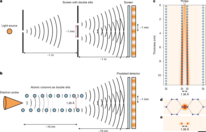
To realize the atomic-scale double-slit geometry, the crystal was precisely oriented to the [110] zone axis using Kikuchi lines and position-averaged convergent beam electron diffraction (PACBED). The electron-probe position at the centre of the Si [110] dumbbell was determined a posteriori with 12-pm precision from the acquired 4D-STEM dataset using a two-step numerical procedure. We note that the high-angle interference fringes used for correlation extraction are inherently robust against small probe positioning offsets, as the fringe visibility is governed by the intercolumn optical-path difference rather than the absolute probe position, and any residual positional uncertainty is already subsumed within the finite effective source size accounted for in the simulations (Supplementary Note 3). First, initial atomic column positions were estimated from the reconstructed annular dark-field images using 2D Gaussian peak fitting (Extended Data Fig. 8a). Then, to overcome precision limits imposed by scan noise and sample drift, we refined the dumbbell centre positions by exploiting the crystallographic symmetry of the CBED patterns³⁸. Using the twofold rotational symmetry (C₂) of the Si [110] projection, we calculated a symmetry score S(r) at each probe position r, defined as 1 minus the normalized MSE between the CBED intensity and its 180°-rotated counterpart:

in which S(r) = 1 (S ∈ [−1, 1]) corresponds to exact twofold rotational symmetry. As shown in Extended Data Fig. 8b, this score exhibits sharp local maxima at high-symmetry points. We identified the refined dumbbell centres by locating these maxima in the vicinity of the coarse estimates. To achieve high signal-to-noise ratios while minimizing the impact of sample drift at each temperature, we acquired several 4D-STEM datasets (typically 10–15 scans within the same tens of nanometres field of view) under identical experimental conditions. For each temperature, equivalent CBED patterns corresponding to the refined dumbbell centres identified across these datasets were extracted and averaged to produce the high signal-to-noise ratio experimental patterns used for quantitative visibility analysis.

In situ heating experiments

Temperature-dependent observations were conducted using the same in situ TEM heating holder. The sample was sequentially heated to 300 K (room temperature), 500 K and 900 K, with sufficient time allowed at each temperature set point to ensure thermal equilibrium before image acquisition. STEM images and 4D-STEM datasets were recorded at each temperature under identical optical conditions to enable quantitative comparison of temperature-dependent changes.

Scattering simulations

CBED patterns were simulated using the multislice method implemented in the abTEM³⁹ code. The microscope parameters were set to match the experimental conditions: an accelerating voltage of 300 kV and a probe-forming aperture semi-angle of 9.1 mrad. The electron probe was positioned at the centre of the Si [110] dumbbell. To account for the finite source size and effective probe instability, we mix adjacent diffraction patterns using Gaussian weights with a FWHM of 0.8 Å as a function of the distance between the probe positions at which the patterns were simulated. No aberrations (defocus, spherical or chromatic) were applied, as the effect of typical residual aberrations was found to be negligible (Supplementary Note 3). The sample thickness for each temperature dataset was determined by maximizing the cross-correlation coefficient between experimental and simulated PACBED patterns⁴⁰ (Extended Data Fig. 9). We confirmed by simulation that whether the left or the right atomic column terminates last at the exit surface makes no notable difference to the resulting patterns (Supplementary Note 10). The estimated thicknesses were 12.7 nm at 300 K, 10.8 nm at 500 K and 10.4 nm at 900 K. For all simulations, thermal diffuse scattering was calculated by averaging over 1,000 frozen-phonon configurations. In the full correlated model, phonon vibrations in all directions are included. Note that atomic displacements parallel to the beam have a negligible first-order effect on the projected potential and hence on the CBED intensities, so the lateral displacements are the dominant factors governing fringe visibility (Supplementary Note 11).

Phonon-displacement models

We used three distinct approaches to model atomic displacements for the frozen-phonon calculations, ranging from independent vibrations to full ab initio-derived correlations.

Independent displacements (Einstein) model: as a baseline for uncorrelated motion, atomic displacements were sampled from isotropic Gaussian distributions with zero interatomic correlation (ρ = 0). The vibrational amplitudes were determined from the full phonon calculations described below to provide a consistent reference for comparison with the correlated model. We used nominal root mean square displacements of \(\sqrt{\langle {u}^{2}\rangle }=0.08\,\mathring{{\rm{A}}}\) at 300 K, 0.10 Å at 500 K and 0.13 Å at 900 K, which are in good agreement with the experimental Si Debye–Waller values tabulated by Peng et al.⁴¹, derived from experimentally determined phonon densities of states.

Full phonon-based correlation model: to capture realistic vibrational correlations of the periodic crystal, we performed phonon calculations. We used a machine-learned Gaussian approximation potential⁴² trained on density functional theory simulations for silicon⁴³. Interatomic force evaluations were performed in QUIP⁴⁴ through its Python interface, quippy⁴⁵. Second-order harmonic force constants were then extracted by means of finite-displacement calculations in a 4 × 4 × 4 supercell using the hiPhive⁴⁶ package, including two-body terms with a cut-off of 4 Å (a higher cut-off or the inclusion of three-body terms did not appreciably alter the results). The calculated phonon dispersion relation derived from these force constants using phonopy^47,48 (Extended Data Fig. 10) shows excellent agreement with established theoretical and experimental data, confirming that the force constants extracted from the Gaussian approximation potential appropriately reproduce the vibrational properties of silicon.

Thermal atomic displacements with correlated phonons were generated by superimposing harmonic normal modes with amplitudes and phases sampled to satisfy canonical ensemble statistics. Correlated displacement snapshots were generated in a 10 × 14 × N_z supercell constructed by repeating the Si [110] conventional unit cell, in which N_z is the supercell dimension along the beam-propagation direction and was set to correspond to the specimen thickness used in the experiment. To account for nuclear quantum zero-point motion, which is non-negligible especially at lower temperatures, we used the QM_statistics option in hiPhive⁴⁶, in which the classical phonon amplitudes are replaced by quantum-statistical harmonic-oscillator amplitudes⁴⁹. Equivalently, this can be written in terms of a mode-dependent effective temperature T_eff (in which ħ is the reduced Planck constant, k_B the Boltzmann constant and ω the mode frequency):

Nearest-neighbour chain model: for parametric studies, we constructed a simplified model that captures the essential physics of nearest-neighbour coupling within the two adjacent Si columns. This model enables us to generate atomic displacements for frozen-phonon simulation at a given temperature using specific correlation coefficients. Although the full phonon calculation involves the entire crystal, we modelled the lattice vibrations along the beam direction effectively as a harmonic chain with nearest-neighbour interactions. In this picture, the cumulative interaction with the surrounding bulk crystal—atoms other than those in the two columns—is renormalized into an effective on-site potential. We separately treated the intercolumn (x) and perpendicular (y) correlated displacements as independent 1D harmonic chains. The effective Hamiltonian is defined by an on-site spring constant K (representing the mean-field stiffness provided by the surrounding lattice) and an interatomic spring constant k (coupling adjacent atoms within the chain):

in which u_α,i represents the displacement of the ith atom along the α ∈ {x, y} axis.

In the language of statistical mechanics, we consider the collective displacement vector u_α = [u_α,1, u_α,2,…, u_α,N]^T for a chain of N atoms. The potential energy term can be written in matrix form as \({{V}}_{\alpha }=\frac{{\rm{1}}}{{\rm{2}}}{{{\bf{u}}}_{\alpha }}^{{\rm{T}}}{{\Phi }}_{\alpha }{{\bf{u}}}_{\alpha }\). Here Φ_α is the tridiagonal force-constant matrix along the α axis, which explicitly takes the form:

Here we assume periodic boundary conditions (or focus on the bulk limit N → ∞), so that each atom has two nearest neighbours along the chain. The diagonal elements (K_α + 2k_α) represent the total stiffness felt by an atom owing to the on-site potential and bonds to both neighbours, whereas the off-diagonal elements (−k_α) represent the coupling. In the classical canonical ensemble, harmonic vibrations at temperature T follow the Boltzmann distribution P(u_α) ∝ exp(−V_α/k_BT), which is mathematically equivalent to a multivariate normal distribution with the precision matrix \({{\varSigma }_{\alpha }}^{-1}={{\Phi }}_{\alpha }/{k}_{{\rm{B}}}T\). The correlation coefficient ρ_α between nearest-neighbour atoms A and B is formally defined as the normalized covariance of their displacements:

in which ⟨…⟩ denotes the ensemble average. Analytical solution of this linear-chain system yields a direct relationship between the correlation coefficient ρ_α and the stiffness ratio κ_α ≡ k_α/K_α:

with the exact inverse relation

This relationship allows us to bridge the statistical and physical pictures: extracting the correlation coefficient from the interference pattern is equivalent to determining the local stiffness ratio κ_α of the atomic bonds. For the frozen-phonon simulations, we generated the displacements of atoms within two Si columns from the multivariate normal distribution defined by the precision matrix \({{\varSigma }_{\alpha }}^{-1}\) derived from ρ_α.

Correlation extraction workflow

To extract the correlation coefficients from experimental data (Fig. 4), we performed a systematic grid search. For each temperature, we simulated CBED patterns on a 41 × 41 grid of (ρ_x, ρ_y) values ranging from 0.0 to 0.8 in steps of 0.02. To specifically isolate the atomic-scale double-slit interference fringes emerging on the thermal diffuse scattering background, we masked out the bright-field disc and the low-angle Bragg diffraction regions (<27.3 mrad). This masking strategy effectively excludes low-angle intensities that are highly sensitive to experimental imperfections (such as residual aberrations and sample mistilt). The agreement between experiment and simulation was evaluated using the MSE of the normalized intensity distributions within this unmasked high-angle region. The optimal parameters were determined by fitting the discrete MSE landscape with a bicubic spline function and finding the global minimum of the function using the L-BFGS-B (ref. ⁵⁰) optimization algorithm implemented in the SciPy (ref. ⁵¹) package. To estimate the statistical uncertainties of the extracted coefficients, we randomly partitioned the total averaged CBED patterns into five independent subsets. The entire extraction procedure was repeated for each subset and the 95% CI for both ρ_x and ρ_y was calculated from the resulting variance. Note that this precision was achieved from a total dose of about 3 × 10⁷ electrons. Because the uncertainty is limited by shot noise and scales with the inverse square root of the dose, and averaging over equivalent pairs simply accumulates dose, tuning the total dose to the precision required for a given problem could make single-position acquisition at an individual column pair feasible.

Spectral analysis of vibrational correlations

To identify which phonon modes contribute to the interference visibility, we decomposed the projected MSRD (see Supplementary Note 4 for derivation) into individual mode contributions and visualized them on the phonon dispersion relation, presented in Extended Data Fig. 7.

In STEM, the electron beam interacts with the atomic potential integrated along the column. To account for this projective geometry, we define the column-averaged projected-mass-normalized eigenvector \({\mathop{{\bf{e}}}\limits^{ \sim }}_{j,{\bf{q}}\nu }\) for atom j (j = A, B for the two columns) in mode (q, ν) as

in which e_j,qν is the phonon eigenvector from phonon calculations, m_j is the atomic mass and R_l denotes lattice translation vectors along the beam direction. The summation runs over N_z unit cells corresponding to the specimen thickness. The Bloch phase factor exp(iq · R_l) determines whether displacements in successive unit cells interfere constructively or destructively in the projected signal.

For directionally resolved analysis (Fig. 4e,h), we extract the Cartesian component α ∈ {x, y}:

in which \({\hat{{\bf{n}}}}_{x}\) is aligned with the Si–Si bond axis and \({\hat{{\bf{n}}}}_{y}\) is perpendicular to it within the imaging plane.

For visualization of the phonon dispersion, we group modes into spectral bins \({{\mathcal{D}}}_{{\bf{q}},\omega }\), defined as the set of modes at wavevector q with frequency within a small window centred at ω. The contribution of each bin to the projected MSRD along direction α is given by:

in which

is the quantum harmonic oscillator amplitude factor, arising from the variance \(\langle {|{\bf{u}}|}^{2}\rangle =\frac{\hbar }{2m\omega }\coth \left(\frac{\hbar \omega }{2{k}_{{\rm{B}}}T}\right)\). For the Si [110] dumbbell structure, inversion symmetry about the bond midpoint ensures \({|{\mathop{e}\limits^{ \sim }}_{A,{\bf{q}}\nu }^{(\alpha )}|}^{2}={|{\mathop{e}\limits^{ \sim }}_{B,{\bf{q}}\nu }^{(\alpha )}|}^{2}\). Under this symmetry, the MSRD contribution factorizes exactly into a thermal population term \({B}_{{\mathcal{D}}}^{(\alpha )}\) (i) and a spectral correlation coefficient term \({c}_{{\mathcal{D}}}^{(\alpha )}\) (ii):

1. (i)

   Thermal population \({B}_{{\mathcal{D}}}^{(\alpha )}\): the thermally excited mean squared displacement is quantified by

   $${B}_{{\mathcal{D}}}^{(\alpha )}({\bf{q}},\omega )=\left(\sum _{\nu \in {\mathcal{D}}}{|{\mathop{e}\limits^{ \sim }}_{A,{\bf{q}}\nu }^{(\alpha )}|}^{2}+\sum _{\nu \in {\mathcal{D}}}{|{\mathop{e}\limits^{ \sim }}_{B,{\bf{q}}\nu }^{(\alpha )}|}^{2}\right)\,A(\omega ).$$

   This quantity represents the vibrational power available from each mode, combining the zero-point amplitude (∝ 1/ω) and thermal occupation. In the high-temperature (classical) limit, the thermal part scales as \({B}_{{\mathcal{D}}}^{(\alpha )}\propto 1/{\omega }^{2}\).

2. (ii)

   Spectral correlation coefficient: the extent to which a mode generates relative displacement between the two columns is quantified by the correlation coefficient:

This coefficient ranges from +1 (perfectly in-phase motion, generating no relative displacement) to −1 (perfectly out-of-phase motion, generating maximum relative displacement). The factor \((1-{c}_{{\mathcal{D}}}^{(\alpha )})\) thus represents the capacity of the mode to induce relative motion between the two columns along direction α.

This factorization confirms the spectral filtering mechanism: marked contribution to the MSRD (and hence to visibility loss) requires both substantial thermal population (\({B}_{{\mathcal{D}}}\) large) and substantial relative-motion capacity (\((1-{c}_{{\mathcal{D}}})\) large).

The mode-resolved analysis is shown in Fig. 4e,h and Extended Data Fig. 7. In Extended Data Fig. 7a,c, the thermal population factor is encoded in the line width of the dispersion curves and the spectral correlation coefficient is shown by the line colour (red: in-phase, \({c}_{{\mathcal{D}}}\simeq 1\); grey: no correlation, \({c}_{{\mathcal{D}}}\simeq 0\); blue: out-of-phase, \({c}_{{\mathcal{D}}}\simeq -1\)). The resulting MSRD contribution W_MSRD is visualized by the colour intensity in Fig. 4e,h and Extended Data Fig. 7b,d, highlighting the modes that dominate visibility loss.