Materials

Chemicals were purchased from commercial suppliers (Thermo Scientific, Merck KGaA, VWR and Honeywell). Solvents and reagents used for peptide synthesis were obtained in peptide grade. Solvents used for peptide purification were of high-performance liquid chromatography (HPLC) grade; dimethyl sulfoxide (DMSO) was BioUltra grade for molecular biology (≥99.5%, Sigma Aldrich); and water was obtained from a Millipore purification system. Dulbecco’s phosphate buffered saline (DPBS; 1x, without CaCl₂ and MgCl₂, composition: KCl 0.2 g l ⁻¹, KH₂PO₄ 0.2 g l ⁻¹, NaCl 8.0 g l ⁻¹, Na₂HPO₄ (anhydrous) 1.15 g l ⁻¹) was purchased from Sigma Aldrich (DPBS) or from Thermo Fisher Scientific (Dulbecco’s balanced salt solution) with minor variations in inorganic salt water content. DILT1 was in part purchased from GenScript Biotech with a purity of ≥98%. DILT2-5 and peptides P1 and P3–P8 were purchased from GenScript Biotech with a purity of ≥98%.

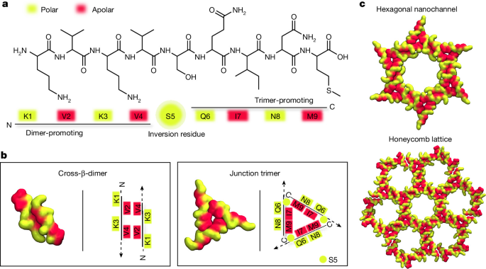
Solid-phase peptide synthesis of DILT1 (KVKVSQINM) and P2 (KLKLSQINM)

For peptide synthesis, the fluorenylmethyloxycarbonyl (Fmoc) solid-phase peptide synthesis strategy was applied from the C-terminus to the N-terminus using N,N′-diisopropylcarbodiimide (DIC) and ethyl cyano(hydroxyimino)acetate (Oxyma) on an automated microwave-assisted peptide synthesizer (CEM, Liberty Blue). The peptides were synthesized onto pre-swollen Fmoc-Met-Wang resin (0.1 mmol, 0.147 g, substitution 0.68 mmol g⁻¹, 100–200 mesh, pre-swollen in dimethylformamide (DMF; 2–3 ml) on a shaker at room temperature) by sequential coupling of activated Nα-Fmoc-amino acid in DMF (2.5 ml, 0.2 M) in the presence of DIC (1 ml, 0.5 M) and Oxyma (0.5 ml, 1.0 M) in DMF via microwave-assisted reaction at 75 °C (170 W) for 15 s and 90 °C (30 W) for 110 s followed by multiple washing of the resin (DMF, 2 × 3 ml, 1 × 4 ml). Sequentially, for DILT1 Fmoc-Asn(Trt)-OH, Fmoc-Ile-OH, Fmoc-Gln(Trt)-OH, Fmoc-Ser(tBu)-OH, Fmoc-Val-OH, Fmoc-Lys(Boc)-OH, Fmoc-Val-OH and Fmoc-Lys(Boc)-OH were coupled to the resin via cycling coupling with each amino acid introduced in one sequential coupling cycle, washing, and Nα-Fmoc-deprotection steps. For P2, Fmoc-Leu-OH was used instead of Fmoc-Val-OH. Nα-Fmoc deprotection was conducted by application of piperidine (3 ml, 20% v/v in DMF) under heating (75 °C, 155 W, 15 s, followed by 90 °C, 30 W, 50 s), followed by washing with DMF (2 × 2 ml, 1 × 3 ml). The synthesized peptides on resin were kept in DMF at 4 °C until further use. Subsequently, the peptides were cleaved from the resin using a cleavage cocktail (10 ml) comprising trifluoroacetic acid (TFA) (95% v/v), Milli-Q water (2.5% v/v) and triisopropylsilane (TIPS) (2.5% v/v). After 2 h incubation on a shaker at room temperature, the peptides were precipitated with diethyl ether pre-cooled to 4 °C (40 ml) and centrifuged at 4,000 rpm for 16 min (×2, 0 °C). The resultant crude products were dried overnight at room temperature. The crude products were purified by preparative reverse-phase HPLC using a 0.1% TFA water–acetonitrile mixture as eluant and lyophilized to yield the peptide as a white amorphous powder. The purified peptides were characterized by matrix-assisted laser desorption/ionization time-of-flight mass spectrometry (MALDI-TOF MS). The lyophilized solids were stored at −20 °C until use.

MALDI-TOF MS (DILT1): m/z_calc = 1,045.60, m/z_found: 1,046 [M + H]⁺, 1,062 [M + O + H]⁺, 1,068 [M+Na]⁺, 1,084 [M + K]⁺, 1,100, 1,106.

MALDI-TOF MS (P2): m/z_calc = 1,073.63, m/z_found: 1,074 [M + H]⁺, 1,090 [M + O + H]⁺, 1,096 [M+Na]⁺, 1,112 [M + K]⁺, 1,128, 1,134, 1,150, 568.

High-performance liquid chromatography

The synthesized crude peptide was purified via preparative HPLC of the dissolved and filtered (0.22 µm) precipitate (Shimadzu system). Multiple manual injections (2× or 3 × 8 mL;) of the peptide crude solution (c = 1.3 mg ml⁻¹, water with 0.1% TFA (v/v) and 5% acetonitrile (ACN) (v/v)) were performed. Separation was performed by a preparative reverse-phase HPLC column (Phenomenex 5 µm C18, 150 × 30 mm) using a 0.1% TFA water–ACN mixture as eluant (flow 25 ml min⁻¹), the applied gradient was as follows: (1) 0.01 min: 5% ACN, 0.1% TFA (A) with 95% 0.1% TFA in water (B); (2) 5 min: 5% A with 95% B; (3) 17 min: 70% A with 30% B; (4) 19 min: 100% A with 0% B; (5) 24 min: 100% A with 0% B; (6) 28 min: 5% A with 95% B; (7) 30 min: 5% A with 95% B. Chromatography was monitored with an ultraviolet absorption detector at 214 nm. Alternatively, the gradient can be applied as follows (for example, P2); (1) 0.01 min: 0% ACN, 0.1% TFA (A) with 100% 0.1% TFA in water (B); (2) 5 min: 0% A with 100% B; (3) 15 min: 40% A with 60% B; (4) 17 min: 100% A with 0% B; (5) 19 min: 100% A with 0% B; (6) 21 min: 5% A with 95% B; (7) 24 min: 5% A with 95% B. Data were evaluated in LabSolutions software.

MALDI mass spectrometry

Peptide mass spectra were recorded in positive ion reflector mode on a Bruker rapifleX MALDI-TOF/TOF mass spectrometer (Bruker Daltonik, scanning smartbeam 3D 10-kHz neodymium-doped yttrium aluminium garnet (Nd:YAG) laser, wavelength of 355 nm, and 10-bit 5-GHz digitizer, acceleration voltage 20 kV) using α-cyano-4-hydroxycinnamic acid (HCCA) as the matrix. Samples were measured with random walk ionization across the sample spot, and usually 8,000 shots were averaged per spectrum. The sample was prepared by mixing an acidic aqueous analyte solution (0.1% TFA) in equal amounts with the supernatant of a saturated HCCA solution acetonitrile/water (30:70 + 0.1% TFA). Subsequently, this mixture (1 µl) was applied to a stainless steel target and allowed to dry before measurement. Calibration was conducted with sodium adducts of polyethylene glycol in a mass range of 500–3,000 Da. Data were evaluated with mMass software.

MSMS sequencing

The sequence analysis was carried out on a rapifleX MALDI-TOF/TOF mass spectrometer from Bruker Daltonik. The instrument is equipped with a scanning smartbeam 3D 10-kHz Nd:YAG laser at a wavelength of 355 nm and a 10-bit 5-GHz digitizer. The acceleration voltage was set to 20 kV, and the mass spectra were recorded in positive ion MSMS mode. The protonated molecular ion of the peptide at 1,046 Da was selected as precursor with an isolation window of +6 Da and −6 Da. Basic instrument calibration was done with the Bruker peptide mix and the Bruker protein calibration standard I and II in a mass range up to 70 kDa. Before fragment ion analysis, the instrument was manually recalibrated with the exact mass of the precursor ion at 1,046.5418 m/z. Samples were measured with random walk ionization across the sample spot. The laser power was adjusted to provide significant signal intensity for b- and y-series fragments, and 2,000 shots were averaged per spectrum. Sample preparation was done by mixing a 50 mg ml⁻¹ solution of super-DHB matrix in acetonitrile/water (1:1 + 0.1% TFA) with equal amounts of the peptide solution (10 mg ml⁻¹) in acetonitrile/water (1:1 + 0.1% TFA). Finally, 1 µl of the mixture was applied to a stainless steel target and allowed to dry before measurement. The mass spectrometer was controlled by the software Bruker flexControl (Version 4.0) and data analysis was done by Bruker flexAnalysis (Version 4.0).

Peptide nanofibril formation

Nanofibril formation was induced by introducing the pre-dissolved peptide stock solution (10 mg ml⁻¹, DMSO) into DPBS (pH 7.4), yielding a 1 mg ml⁻¹ solution. After brief vortexing, the samples were incubated on a shaker (500 rpm, room temperature) overnight. Further incubation was conducted as indicated without shaking at room temperature or at 37 °C for the indicated periods.

Peptide nanofibril electron microscopy screening

Cryo-EM

For cryo-EM micrograph screening of DILT2–DILT5 and peptides P1 and P3–P8, samples were incubated as described above (1 mg ml⁻¹) overnight (500 rpm, 25 °C), subsequently kept at room temperature without shaking and plunge-frozen after 4 days. Holey-carbon-coated grids (400 mesh C-flat 1.2/1.3) were glow-discharged (PELCO easiGlow glow discharge cleaning system; TED PELLA), 3 µl sample was applied, blotted for 8 s and plunge-frozen in liquid ethane using an Automatic Plunge Freezer EM GP2 (Leica Microsystems) for each sample. Grids were screened on a JEM-2100 transmission electron microscope (Jeol) at 200 kV using a TVIPS F416 camera.

Transmission electron microscopy

P2 (L2/L4) was imaged after overnight incubation via TEM as described previously^42,43. The pre-incubated sample (5 μl, 1 mg ml⁻¹) was placed on a copper grid coated with formvar layer (etched with oxygen plasma). Following a short incubation, excess liquid was removed with filter paper, and the grids were stained with uranyl acetate solution (4% w/v, 2 min) and washed with water. Measurements were performed on a Jeol 1400 electron microscope with 120 kV acceleration voltage.

Cryo-EM sample preparation and data acquisition

For DILT1 analyses, samples were incubated overnight (500 rpm, 22 °C), and further sample incubation was conducted without shaking at 37 °C for the indicated periods. For DILT2 (2-2-2) and DILT3 (2-2-2) cryo-EM reconstruction analyses, samples were incubated overnight (500 rpm, 25 °C), subsequently kept at 37 °C without shaking, and plunge-frozen after 7 days and 1 day, respectively. In case of DILT1 and DILT3, a 4 µl aliquot of the DILT1 fibril sample (from the indicated incubation time points) was applied on a Quantifoil grid (Q R2/2, 400 mesh) that was glow-discharged in a 6:1 oxygen/hydrogen plasma (Diener Nano, Diener Electronic) for 30 s shortly before. The excess solution was blotted for 4 s at 4 °C and >80 % humidity. The specimen was cryo-plunged in liquid ethane using a Vitrobot Mark V (Thermo Fisher Scientific). Subsequent imaging was done using a Titan Krios G4 transmission electron microscope (Thermo Fisher Scientific) at 300 kV, equipped with a Gatan GIF continuum spectrometer. Micrographs and videos were acquired on a 6,912 × 6,912-pixel K3 Gatan direct electron-detection camera with the spectrometer operated in imaging mode using a slit width of 20 eV. For data acquisition, the K3 camera was operated in super resolution and correlated double sampling mode. Extended Data Table 1 lists the data acquisition parameters.

For DILT2 (4-4-4) and DILT3 (3-3-3) cryo-EM reconstruction analyses, samples were incubated overnight (500 rpm, 25 °C), subsequently kept at room temperature without shaking, and plunge-frozen after 15 days for DILT2 and after 8 days for DILT3. For each, 3 µl of sample was applied to a glow-discharged (PELCO easiGlow glow discharge cleaning system; TED PELLA) holey-carbon-coated grid (400 mesh C-flat 1.2/1.3). After blotting with filter paper for 8 s and plunge-freezing in liquid ethane using an Automatic Plunge Freezer EM GP2 (Leica Microsystems), the grids were screened on a JEM-2100 transmission electron microscope (Jeol) at 200 kV, equipped with a TVIPS F416 camera. The dataset for reconstruction was recorded on a Krios G4 transmission electron microscope (Thermo Fisher Scientific) with a Falcon4i (Thermo Fisher Scientific) direct electron detector and a Selectris X energy filter (Thermo Fisher Scientific) operated with a 10-eV slit width. Extended Data Table 1 lists the data acquisition parameters.

Helical reconstruction

In the case of DILT1 fibrils, MotionCor2⁴⁴ was used for movie correction. Contrast transfer function (CTF) for all micrographs was performed using CTFFIND⁴⁵. Further image processing and 3D helical reconstructions were performed with RELION-4.0^46,47 on the 1-1-1 (hexagon fibril) and 3-3-3 (honeycomb fibril) morphologies. For the 3-3-3 morphology, micrographs containing ice or lacking the 4.8-Å-resolution information were excluded. The 3-3-3 morphology filaments were manually picked. As an initial model for the refinement, a featureless cylinder was used with a 60-Å low-pass filter and C₁ symmetry. From the 3D auto-refinement, a C₆ symmetry was observed and imposed, reaching a 4.3-Å-resolution volume with clearly visible β-sheets. To further improve resolution, the full dataset was re-processed via 3D classification and further 3D auto-refine to reach the final 3 Å volume. The volume was then post-processed with a soft-edge mask and sharpened with a B-factor of −50. All 3D classifications were carried out on the central 10% of the reconstruction. For the 1-1-1 morphology, a similar approach was performed. Details of particle extraction and helical reconstruction are reported in Extended Data Table 1.

In the case of the 2-2-2 DILT2 fibrils, CTF for all single images, acquired with drift correction in SerialEM, was performed using CTFFIND⁴⁵. Further image processing and 3D helical reconstructions were performed with RELION 5.0⁴⁶. The 2-2-2 morphology filaments were manually picked. As an initial model for the refinement, a simulated 2-2-2 hexagonal morphology was used. From the 3D auto-refinement, a C₃ symmetry was imposed. The volume was then post-processed with a soft-edge mask and sharpened with a B-factor of −50. All 3D analyses were carried out on the central 10% of the reconstruction.

In the case of DILT2 (4-4-4), helical reconstruction was performed in RELION 5.0⁴⁶. Raw video frames were aligned and corrected for beam-induced motion using RELION’s own implementation of MotionCorr2⁴⁴, followed by CTF estimation using CTFFIND 4.1⁴⁵. Fibrils displaying the 4-4-4 morphology were manually selected from the micrographs. Binned segments were extracted and subjected to reference-free two-dimensional classification until a homogeneous set of particles was obtained. Selected segments were extracted for 3D refinement without binning for 3D reconstruction. Helical refinement was performed using a low-passed cylinder and helical twist estimated from the raw micrographs by manual measurement in Fiji⁴⁸, and a helical rise of 4.75 Å without the imposition of rotational symmetry. For the purpose of map improvement, rotational symmetries C₂, C₃ and C₆ were imposed in the subsequent refinement, of which C₃ symmetry yielded the best quality map as validated by visual inspection. Furthermore, the local search for helical parameters was turned on to optimize the twist and rise of the fibril. After the initial reconstructions, 3D classification and selection of the refined particle stack with progressive increase of the Tau fudge factor were carried out to remedy residual heterogeneity. The resulting particles were subjected to Bayesian polishing. The polished, final stack underwent two cycles of CTF refinement and reconstruction until no further improvement of the reconstructed map was noticeable. The final map was masked with a soft-edged mask and post-processed, yielding a map with a nominal gold-standard resolution of 1.9 Å.

In the case of DILT3 (3-3-3), image processing was performed in cryoSPARC 4.7.1⁴⁹. Raw video frames were aligned and corrected for beam-induced motion using cryoSPARC’s internal patch motion correction. CTF parameter estimation was performed by patch CTF estimation. Exposures were manually curated to exclude micrographs with thick ice and fibril overcrowding. Filament segments were automatically picked using the filament tracer, and segments were extracted with binning for initial classification. Reference-free two-dimensional classification was used to separate segments belonging to different fibril morphologies. Particles corresponding to the 3-3-3 morphology were re-extracted without binning. The resulting stack was subjected to multiple rounds of two-dimensional classification to remove low-quality particles. An initial 3D helical reconstruction was performed using a featureless cylinder without the imposition of helical symmetry. The obtained map was used to bootstrap a 3D helical refinement with enforcement of helical symmetry parameters as obtained by measurement in Fiji⁴⁸. Three-dimensional classification without particle alignment was used to resolve structural heterogeneity. Classes displaying clear separation of fibril layers along the helical axis were selected, and helical symmetry search was enabled during subsequent reconstructions. The homogeneous particle stack was subjected to reference beam motion correction in cryoSPARC and subsequent local and global CTF refinements. Several rounds of local CTF refinement and helical refinement were performed until no further improvement of the 3D map was observable. The final particle stack was symmetry expanded, and a final local refinement with recentring was performed. The resulting half-maps and reconstruction mask were imported into RELION 5.0⁴⁶ where masking and post-processing were performed, yielding a final map with a gold-standard resolution of 1.78 Å. Details of particle extraction and helical reconstruction are reported in Extended Data Table 1.

Atomic model building and refinement

In the case of DILT1, the atomic model for morphology 3-3-3 was built de novo using the program Coot⁵⁰. Given the large number of chains present in the structure, model building was performed stepwise. The fundamental chains of the fibril are termed I.II.III–IV.V.VI–VII.VIII–IX.X (Extended Data Fig. 2g). Initially three chains (I-II-III) were constructed in Chimera⁵¹ by applying the standard β-parallel parameters ((Φ, Ψ) = (–135°, 135°)). These were manually aligned to the junction motif in the 3D volume. Next, to limit atomic clashes in the fibril axis, three layers of such chains were constructed. The three-layer system was refined further in Coot⁵⁰ and Chimera⁵¹. An iterative optimization process was performed to achieve optimal fitting. Next, the structure was further extended to take into consideration the cross-β-motif. Once the I-II-III chains were optimized, they were imposed on the remaining outer electron density. MolProbity⁵², the comprehensive validation tool in Phenix⁵³, was used to produce a validation of the atomic model to assess atomic clashes, rotamer and Ramachandran outliers, and model geometry. The structural statistics for refinement and model building are listed in Extended Data Table 1 and refer to the deposited atomic model (18 chains and 3 layers).

In the case of 2-2-2 DILT2 fibrils, the starting model for refinement was the atomic model of DILT1, and the applied rotational symmetry was C₃. The structural statistics for refinement and model building are listed in Extended Data Table 1 and refer to the deposited atomic models.

In the case of DILT3 fibrils, an initial atomic model was generated de novo using ModelAngelo⁵⁴. An iterative model refinement process was used in which an asymmetric unit of a single layer of the C₆-symmetrical DILT3 fibril cross-sections was refined in WinCoot 1.1.18⁴⁹. Phenix 2.0.5936⁵³ was used to evaluate model geometry and clash score. ChimeraX 1.10⁵⁵ was used to obtain a helical assembly of three layers, which was again validated. The three-layer model was further manually refined in WinCoot 1.1.18⁴⁹ using regularization with Ramachandran, torsion and planar peptide restraints, followed by a subsequent real-space refinement. ISOLDE⁵⁶ was used to improve the clash score. After each model refinement cycle, the contact sites between asymmetric units were checked for steric clashes by symmetry expansion to the original fibril symmetry and renewed validation in Phenix. Final images were produced using Fiji⁴⁸ and ChimeraX⁵⁵.

In the case of DILT2 fibrils, the same procedure was used as for DILT3 fibrils, with the exception of the starting model and the applied symmetry. The starting model for refinement of DILT2 was the atomic model of DILT3, and the applied rotational symmetry was C₃. The structural statistics for refinement and model building are listed in Extended Data Table 1 and refer to the deposited atomic models.

Polymorphism analysis

The CTF-corrected micrographs were used for the polymorphism analysis. A subset of 100 micrographs was randomly generated with the RELION ‘Subset Selection’ function. Each of these micrographs was analysed, and the different morphologies were manually picked and extracted using a box size of 350 pixels, nanochannel diameter of 220 Å, number of asymmetric units 7 and rise of 4.7 Å. The number of extracted particles was used to quantify the different morphologies. The polymorphism prediction was performed using Chimera⁵¹, RELION-4.0⁴⁷ and Fiji⁴⁸. Three layers of the atomic model of the central hexagon obtained from the 3-3-3 morphology were copied and shifted manually to create plausible hexagonal patterns. In Chimera⁵¹, the atomic model was converted into a volume with a 3-Å resolution (molmap #0 3) and saved as an .mrc file. The file was then processed with RELION-4.0⁴⁷ to create a prolonged volume. Specifically, the file was converted into a file with a box size of 1,750 pixels, a nanochannel diameter of 250 Å, a rise of 4.77 Å and a twist of −0.64°. The following commands were used:

relion_image_handler–i 2Hex_221.mrc–new_box 1750–o 2Hex_221_BS1750.mrc
relion_helix_toolbox –impose–i 2Hex_221_BS1750.mrc–o 2Hex_221_BS1750_4.77_t0.64.mrc–cyl_outer_diameter 230–angpix 0.8875–rise 4.77–twist -0.64–z_percentage 0.1

The volume was then processed in Fiji⁴⁸. The central 1,511 slices of the volume (which correspond to the number of slices that generate a single crossover distance) were analysed to visualize the projection. To visualize the full 360° rotation pattern, the images were rotated by 180°, and the 2 projection images were combined.

Simulation details

Simulations were performed using the GROMACS 2021.7⁵⁷ molecular dynamics package in the isothermal–isobaric NPT ensemble. The temperature was imposed using a velocity rescale thermostat⁵⁸ at 298.15 K with a time constant of 1.0 ps⁻¹. The pressure was controlled at 1.0 bar using the Parrinello–Rahman barostat⁵⁹ with a time constant of 2.0 ps⁻¹. The equations of motion were integrated using the leap-frog algorithm with a time step of 1.0 fs. Peptide chains and sodium, potassium and chloride ions were modelled using CHARMM36m force-field parameters⁶⁰, and water was described by the TIP3P model^61,62. The H₂PO₄⁻ and HPO₄²⁻ ions parameters were taken from CHARMM FF on CHARMM-GUI^63,64. Electrostatic interactions were treated using the smooth particle mesh Ewald method⁶⁵. The solvent molecules and ions were equilibrated by the steepest descent energy minimization with a tolerance of 100.0 kJ mol⁻¹, with position restraints in all peptide atoms, followed by 25 ns of molecular dynamics simulation with position restraints only in the backbone atoms of the peptides. After the equilibration of the solvent, the systems were simulated for 100 ns without restraints. All simulations were performed on RAVEN HPC at Max Planck Computing and Data Facility, Garching, Germany.

Molecular dynamics analysis

All analyses were performed with the GROMACS 2021.7 molecular dynamics package⁵³. The RMSF was calculated by residue and averaged over time and layer. The size-independent comparison of the 3D structures was done using the scaled dissimilarity index proposed by Maiorov and Crippen⁶⁶. The trajectories were least-squared fitted to the first snapshot of the simulation, using its backbone atoms as reference. The visualization and simulation snapshots were generated with visual molecular dynamics⁶⁷.

DILT1 fibril integrity and solvent interaction

A DILT1 fibril in explicit solvent, consisting of 94 layers with each layer rotated by −0.64° (total twist approximately 60°) was simulated to investigate its integrity. The fibril extends across the 22.0 × 22.0 × 44.8 nm³ simulation box along the z direction, forming an infinitely periodic fibril owing to periodic boundary conditions. The system composition was determined using the systematic equilibrium treatment described previously. The final composition includes: 1,692 peptide chains, 4,739 Cl⁻, 18 H₂PO₄⁻, 96 HPO₄²⁻, 44 K⁺, 1,521 Na⁺, 14,637 DMSO and 509,721 H₂O.

Composition of the system for molecular dynamics

The integrity of the DILT1 junction and cross-β-motif was studied by simulating 1-, 3-, 5-, 10- and 15-layer models for each motif. The same number of layers was simulated to verify the conformational persistence of the hexagon fibril. The layer structures were generated by rotating and translating the fundamental junction unit along the z direction. The geometric centre of the peptides was placed in a 22.0 × 22.0 × 22.0 nm³ simulation box and solvated with a 9:1 (% v/v) mixture of PBS and DMSO.

The system composition was determined from equilibrium calculations at 298.15 K based on the procedure described in ref. ⁶⁸. The dissociation constants of ionizable amino acids (for example, lysine, pK_a = 10.82) were assumed to be independent of each other. Activity coefficients were computed using the temperature-dependent extended Debye–Hückel equation⁶⁸. The experimental value of the dielectric constant of the water/DMSO mixture, needed to obtain the system composition, was obtained from ref. ⁶⁹, corresponding to 78.08 at 298.15 K.

The equilibrium composition of each system was computed numerically using the Newton–Raphson method, with the change in pH, ΔpH <10⁻⁷, as the convergence criterion.

Structure–property relationship simulations

As we have observed that 15 layers are a persistent fibril fragment for DILT1, we have generated samples for the other sequences, DILT2–DILT5, and P1 and P4, with this number of layers. Once the peptide sequence has been mutated in PyMOL, systems were built as before, starting from a junction and applying the corresponding symmetry operations, and simulated following the protocol described above.

DILT 1 nanofibril characterization

The incubation times and temperatures were varied as indicated below for kinetics and stability (solvent, temperature, sonication) characterizations as follows. (1) Preformed fibrils (1 mg ml⁻¹, 10% v/v DMSO, 90% v/v PBS) were obtained by incubating at 22 °C for 24 h with 500 rpm shaking (Extended Data Fig. 7a). (2) Nanofibril formation without pre-dissolved DMSO peptide stock was determined by dissolving the lyophilized peptide directly in DPBS (pH 7.4) yielding a 1 mg ml⁻¹ solution (Extended Data Fig. 7b). (3) A dilution stability test was performed on the preformed fibrils as described in (1), which were incubated at 37 °C for 1 week. The fibrils were then diluted in water. Specifically, 10 μl of the preformed fibrils (1 mg ml⁻¹) was added to 90 μl Milli-Q H₂O (0.1 mg ml⁻¹) with a final composition of 1% v/v DMSO, 9% v/v PBS and 90% v/v Milli-Q H₂O. The sample was incubated for 3 days at 37 °C (Extended Data Fig. 7c). This sample was used for the reconstruction of the 1-1-1 morphology (#2; Extended Data Table 1). (4) Early kinetics experiments were conducted by inducing nanofibril formation via the general method with incubation (22 °C, 500 rpm) for either 30 min, 45 min, 1 h, 3 h, 6 h, 9 h, 15 h, 21 h or 24 h (Extended Data Fig. 7k–s). (5) Late kinetics experiments were conducted using the preformed fibrils as described in (1) and transferring them into a 37 °C oven without shaking. The samples were then imaged after 4 days, 1 week, 2 weeks and 53 days (Extended Data Fig. 7t–w). The 53-day sample was used for reconstruction of the 3-3-3 morphology and for the polymorphism analysis (Extended Data Fig. 2). (6) Temperature stability tests were performed by using the preformed fibrils as described in (1) and transferring them for 15 min or 60 min in an oven at 60 °C, 85 °C or 95 °C (Extended Data Fig. 7d–i). (7) Sonication stability tests were performed by exposing preformed fibrils as described in (1) to sonication (15 min, sonication bath) (Extended Data Fig. 7j).

To minimize contamination during long-term incubation, peptide assemblies were prepared from fresh stock solutions using sterile-filtered buffer and clean consumables; full-grid cryo-EM mapping of long-incubation samples did not reveal contaminating micrometre-scale objects.

Atomic force microscopy

For atomic force microscopy (AFM) screening of DILT1–DILT5 and P3 samples were prepared by introducing the pre-dissolved peptide stock solution (10 mg ml ⁻¹, DMSO) to DPBS (pH 7.4), yielding a 1 mg ml⁻¹ solution, and analysed after overnight incubation (500 rpm, 25 °C, DPBS, pH 7.4). For imaging the DILT and P3 architectures, a Bruker Dimension FastScan BioTM atomic force microscope was used in the liquid state, which was operated in PeakForce mode. FastScan-D tips from Burker with a nominal spring constant of 0.25 Nm⁻¹ were used.

For AFM sample preparation, the pre-incubated peptide solution (100 µl, 1 mg ml⁻¹) was added to a circular mica substrate (20 mm) and incubated for 15 min. The excess liquid was removed, washed with 200 µl buffer (DPBS, pH 7.4), excess liquid was removed and 300 µl buffer was added to the mica to measure in liquid. Images were analysed with NanoScope Analysis 1.9.

In situ humidity-controlled FTIR experiments

Nanofibril formation was induced either by dissolving the DILT1 solid powder directly in the DPBS to yield a 1 mg ml⁻¹ solution (DILT1, Fig. 6e and Extended Data Fig. 9b,e–h) or, alternatively, peptide nanofibril formation was induced as described above by introducing the pre-dissolved peptide stock solution (10 mg ml⁻¹, DMSO) to DPBS (pH 7.4), yielding a 1 mg ml⁻¹ solution (DILT 5, Fig. 6e; DILT 2, Extended Data Fig. 9c; DILT 4, Extended Data Fig. 9d). The same protocol was applied for the control-peptide CKFKFQF. After overnight incubation (500 rpm, 25 °C), DILT1, DILT2, DILT4, DILT5 and CKFKFQF samples, were submitted to in situ humidity-controlled FTIR experiments, respectively. FTIR spectra were recorded in transmission mode using a Bruker VERTEX 70 spectrometer. The spectrometer was purged with nitrogen and all measurements were conducted at room temperature. The pre-incubated peptide samples were loaded into a Teflon flow cell fitted with CaF₂ windows (1 mm thickness) and a 2 mm path length; the sample (approximately 8 µl) was applied with a thickness ≤0.1 mm. The flow cell was mounted in the spectrometer sample compartment and connected to a dry-nitrogen supply to initiate and control dehydration. Spectra were recorded at regular intervals throughout the drying process, which proceeded until no further spectral change indicated complete desiccation.

Estimation of the number of water molecules per peptide

The number of water molecules per peptide was estimated using the known infrared absorption cross-sections of the respective functional groups. Molar extinction coefficients of ϵ_N–H = 100 M⁻¹ cm⁻¹ for the peptide N–H (ref. ⁷⁰) and ϵ_O–H = 400 M⁻¹ cm⁻¹ for the O–H stretch of water molecules⁷¹ were applied. Considering four N–H groups per peptide and two O–H bonds per water molecule, the integrated intensity ratio satisfies \(\frac{Keep following us for the latest insights._{Check back often for more exciting news!-{\rmFor more tech updates, stay tuned to our blog.}}}{{I}_{{\rm{O}}-{\rm{H}}}}\approx \frac{{N}_{{\rm{N}}-{\rm{H}}}\times {{\epsilon }}_{{\rm{N}}-{\rm{H}}}}{2{N}_{\mathrm{water}}\times {{\epsilon }}_{{\rm{O}}-{\rm{H}}}}\), where N_N–H is the number of peptide N–H groups and N_water is the number of water molecules.

For DILT1, after about 110 min in dry nitrogen, the N–H peak at 3,277 cm⁻¹ shows an integrated intensity of 0.15, and the broader water O–H band centred at 3,300 cm⁻¹ shows an integrated intensity of 7.5, corresponding to approximately 25 water molecules per peptide, assuming negligible contribution from backbone N–H groups (Extended Data Fig. 9b). Considering the channel geometry (0.48 nm peptide-layer height, 6 peptides per layer, 5 nm channel diameter) and a water density of 1.05 g cm⁻³ from simulations, a fully filled channel would contain about 55 water molecules per peptide. The FTIR-derived estimate is inherently approximate, as it relies on extinction coefficients from related systems and does not account for peptide side-chain O–H or N–H contributions. Nevertheless, the number inferred from the infrared spectral intensities is consistent with fully filled tubes at about 100 min drying time inferred from the convergence of the spectral shape at that time.

In situ dehydration Raman spectroscopy and Cryo-EM experiments

In situ Raman spectra were recorded using a WITec alpha300 Raman microscope equipped with a 532-nm excitation laser. The laser power at the sample was set to 5 mW. The pre-incubated peptide samples (1 mg ml⁻¹, directly dissolved in DPBS, 500 rpm overnight shaking, 25 °C) were loaded into a Teflon flow cell fitted with CaF₂ windows (1 mm thickness) and a 2 mm path length; the sample, approximately 8 µl, was applied with a thickness ≤0.1 mm. The flow cell was fixed on the microscope sample stage and connected to a dry-nitrogen supply, allowing dehydration to be initiated and controlled during Raman acquisition. Spectra were recorded at regular intervals throughout the drying process until no further spectral changes were observed, indicating complete desiccation.

For cryo-EM analysis after controlled drying, a similarly pre-incubated peptide sample was dehydrated using the same Teflon flow-cell and dry-nitrogen protocol as used for the Raman and FTIR experiments. After approximatey 120 min of drying, the flow cell was opened and a TEM grid was dripped into the residual sample liquid on the CaF₂ window and the TEM grid was then immediately plunge-frozen using a Vitrobot Mark V for subsequent cryo-EM examination.

Characterization of concentration-dependent self-assembly of DILT1

Sample preparation and incubation

DILT1 solutions of various concentrations were prepared. For this, a DILT1 10 mg ml⁻¹ DMSO stock solution, prepared in filtered DMSO, was diluted to yield DILT1 DMSO stock solutions at varying concentrations. Subsequently, these pre-dissolved DILT1 DMSO stock solutions were introduced to DPBS (pH 7.4) in a 1:9 ratio, respectively, yielding solutions with varied concentrations (1,000 µg ml⁻¹, 500 µg ml⁻¹, 100 µg ml⁻¹, 50 µg ml⁻¹, 35 µg ml⁻¹, 17.5 µg ml⁻¹, 8.8 µg ml⁻¹, 4.4 µg ml⁻¹, 2.2 µg ml⁻¹, 500 µl, 10% v/v DMSO in DPBS). The respective samples were mixed by brief vortexing and incubated on a shaker (500 rpm, room temperature) overnight. The given values were accurately rounded up to the full number in Extended Data Fig. 8.

Vial flip test

After overnight incubation of the DILT1 samples (2–1,000 µg ml⁻¹, 10% v/v DMSO in DPBS, 500 µl), the macroscopic gelation behaviour of DILT1 at varied concentrations was examined by vial flip test.

Proteostat assay

The critical aggregation concentration of the DILT1 peptide was examined via the commercial Proteostat protein aggregation assay kit by Enzo Life Sciences. Following the manufacturer’s recommendation, adapting a previously published protocol⁷², the Proteostat working solution was prepared by diluting Proteostat stock solution (0.50 µl) and assay buffer (1 µl 10x assay buffer) in 98.5 µl Milli-Q water. To conduct the assay, 36 μl pre-incubated DILT1 peptide solutions at various concentrations (2–1,000 µg ml⁻¹, 10% v/v DMSO in DPBS) were mixed with 4 μl Proteostat working solution. The samples were transferred into a Greiner 384 flat black well plate (3 wells per sample (technical replicates n = 3), that is, per peptide concentration, 9 µl sample per well), incubated in the dark (15 min) while shaking, and the fluorescence intensity of the Proteostat dye was determined λ_excitation = 550 nm, λ_emission = 600 nm; bandwidths 20 nm, multiple reads per well, respectively. At high DILT1 concentration (956 µM), the aggregation affected sample loading to a maximum of 2 wells, each containing 9 µl of the mix (n = 2).

Transmission electron microscopy

To analyse the aggregate and assembly morphologies at various concentrations, the incubated DILT1 sample solutions (2–1,000 µg ml⁻¹, 10% v/v DMSO in DPBS) were submitted to TEM analysis. Grid preparation was carried out as follows. Five microlitres of the sample solution was deposited onto a TEM grid and allowed to stand for 5 min to enable adequate adsorption. Excess solution was then gently removed using filter paper. Subsequently, staining was performed with 5 µl of 4% w/v aqueous uranyl acetate for 2 min. After staining, the grids were rinsed three times with Milli-Q water to remove excess stain. Finally, the water was gently removed from the grid with filter paper, and the grids were left to dry overnight before TEM measurement. TEM was measured at 120 kV.

Hydrogel and honeycomb fibril preparation

Hydrogels were prepared by either pre-dissolving the DILT1 peptide in DMSO (10 mg ml⁻¹) and adding this DMSO peptide stock solution into DPBS to yield a 1 mg ml⁻¹ solution (0.1 wt%) or by dissolving solid DILT1 powder directly in the respective solvent to yield 1–4 wt% hydrogels. For example, 0.3 mg peptide was dissolved in 30 µl buffer (for example, DPBS, pH 7) and mixed for approximately 5 s to yield a 1 wt% (10 mg ml⁻¹) hydrogel. Very soft hydrogels were obtained at 0.1 wt%, for example, by the nanofibril-formation procedure described in ‘Peptide nanofibril formation’.

Rheology

Rheological characterization was conducted using a DHR3 rheometer (TA Instruments) equipped with a temperature controller and a solvent reservoir to prevent hydrogel drying. Experiments were performed using an 8-mm parallel-plate geometry with hydrogels of approximately 30 μl volume (gap size of about 0.5 mm). Characterization of the hydrogel mechanical properties was conducted at 25 °C. Gels were prepared directly on the plate by the procedure described in ‘Hydrogel and honeycomb fibril preparation’. Oscillatory time-sweep measurements monitored the gelation at a fixed strain of 0.1% and a fixed frequency of 1 Hz. Extended Data Fig. 8e presents representative sections after complete gelation (approximately last 300 s of gelation curves), which summarizes individual measurements recorded with time stamps at approximately 6-s intervals (time stamps are indicative). Oscillatory strain sweeps (0.01–200% or 0.01–1000%, as indicated) were conducted at a fixed frequency of 1 Hz. Oscillatory frequency sweeps (0.05–100 Hz) were performed at a fixed strain of 0.1%.

DILT1 gel stability

Photographs were taken with a Canon EOS 250D with a Canon EF 24–105 mm f/4L IS lens. Manual mode, exposure of 1/50 with aperture of f/8 and focal length of 105 mm. ISO 100. Saved in jpg format with a resolution of 5,284 dpi.