In this study, we combine century-scale river chemistry records, reconstructed acidity and alkalinity inputs, and reactive transport simulations to evaluate whether agricultural liming in the MRB has acted as a net CO₂ source or sink. We use existing long-term discharge and alkalinity flux records²¹ to estimate excess riverine alkalinity export relative to a pre-1935 baseline. Separately, we compile long-term estimates of Ca and Mg (and SO₄²⁻ as well as NO₃⁻ + NO₂⁻) concentrations for the Lower Mississippi River and combine these with existing bicarbonate data to estimate the fraction of carbonate weathering driven by strong acids rather than carbonic acid, following the approach outlined in ref. ¹⁷. We then build a spatially explicit acidity–alkalinity budget for the MRB, including alkalinity inputs from agricultural lime and acidity inputs from fertilizer, manure, SON mineralization, agricultural BNF, and atmospheric S and N deposition. Finally, we use the reactive transport model SCEPTER^36,51,52 to evaluate how these reconstructed acid and alkalinity inputs interact with carbonate dissolution, cation exchange and hydrologic export, and to compare acidity-only counterfactual simulations with simulations that include historical liming. The sections below describe the procedures used to estimate acidity and alkalinity inputs from each source and underlying dataset, the river-flux and strong-acid-weathering calculations, and the SCEPTER model set-up. Uncertainty propagation for all calculations is described in the dedicated uncertainty section at the end. More information can be found in Supplementary Information.

Solute concentrations in the MRB

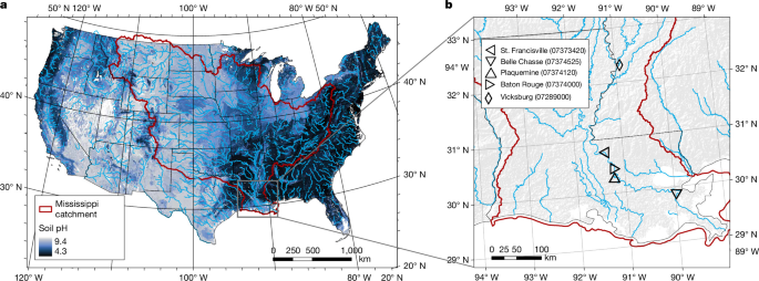
The MRB data analysed here build on concentration measurements from five US Geological Survey stations⁵³ (Fig. 1 and Supplementary Fig. 1) spanning over seven decades, as well as published data from the early 1900s^54,55 and long-term time series of Mississippi discharge and total alkalinity titrations (assumed to be equivalent to HCO₃⁻ concentrations)^21,22. Annual flow-weighted average concentrations for Ca (combining US Geological Survey parameters 00915 and 00916), Mg (00925 and 00927), SO₄²⁻ (00945) and NO₃⁻ + NO₂⁻ (00631) were calculated based on the data from five stations (Fig. 1): Mississippi River at Vicksburg, MS, station 07289000; Mississippi River at St. Francisville, LA, station 07373420; Mississippi River at Baton Rouge, LA, station 07374000; Mississippi River at Plaquemine, LA, station 07374120; Mississippi River at Belle Chasse, LA, station 07374525.

Although reported as total dissolved Ca and Mg, throughout this paper, we assume that these quantities are dominated by their dissolved ionic forms (Ca²⁺ and Mg²⁺). Owing to their similar watersheds and to maximize temporal coverage, data from these five stations were combined and monthly average concentrations were calculated. Using monthly discharge data²¹, annual flow-weighted averages were calculated. The calculated annual average concentrations are shown in Supplementary Fig. 1 and briefly discussed in Supplementary Information, section 1.1. Because daily and/or instantaneous discharge data are lacking for most of the record, robust estimation of concentration–discharge (C–Q) relationships across the full time series is not possible. Although C–Q approaches would in principle provide additional resolution, their application would require combining heterogeneous and discontinuous datasets, which introduces substantial uncertainty. We therefore use flow-weighted annual concentrations as the most internally consistent method for capturing long-term trends. To estimate the increase in riverine bicarbonate fluxes relative to the pre-liming baseline, we use published estimates of annual bicarbonate flux²¹, calculate the average pre-1935 flux as a baseline state and define post-1934 excess fluxes relative to this baseline. Missing post-baseline years in the published record (1942–1944, 1955 and 1966–1968) are gap-filled by linear interpolation between pre- and post-gap anchor values calculated as 3-year means of the nearest available years on either side of each gap, which does not materially change the results compared with omitting these years (Supplementary Information, section 1.2 and Supplementary Fig. 6).

Considering the stoichiometry of carbonate mineral dissolution by reaction with carbonic acid at circumneutral pH, excess riverine bicarbonate fluxes are converted to lime CDR assuming that half of the associated carbon is derived from the atmosphere and half is derived from carbonate minerals. Riverine transported lime-derived CDR is therefore estimated by converting 50% of excess (molar) alkalinity fluxes into metric tons of CO₂. To isolate the effect of liming on riverine alkalinity fluxes, we also explore accounting for hydroclimate-driven changes in baseline weathering by incorporating historical temperature trends and water-flux constraints based on precipitation and precipitation minus evapotranspiration (P−ET) using established weathering–hydroclimate scaling relationships⁵⁶. These adjustments primarily broaden the uncertainty range of excess riverine alkalinity export rather than substantially altering its central estimate or sign (Supplementary Information, section 1).

The focus on the lower Mississippi River reflects the availability of a uniquely continuous, century-scale record of discharge and alkalinity^21,22, which enables resolution of multi-decadal responses to liming and acidification. Comparable records are not available for most sub-basins, where discontinuities in monitoring and limited historical coverage preclude robust reconstruction of long-term carbon fluxes, pre-liming baselines and lag times. As a result, the basin-scale outlet provides the most reliable constraint on integrated carbon export dynamics over the timescales considered here. This long-term perspective is essential for resolving the decadal-scale lag between lime application and alkalinity export, which cannot be robustly constrained using shorter or discontinuous sub-basin records.

Quantifying strong-acid weathering

Our approach to quantifying the fraction of lime dissolved as a result of reaction with strong acids rather than carbonic acid builds on the approach of comparing water Ca²⁺ and Mg²⁺ concentrations (in meq l⁻¹) with water HCO₃⁻ concentrations (in meq l⁻¹) as developed by ref. ¹⁷ (Extended Data Fig. 1). Previously, this approach was applied to soil solutions, tile drainage and stream water¹⁷. Here we assume that this framework also applies to the Mississippi watershed because the majority (approximately 58%) of the catchment is covered with croplands⁵⁷ and overall riverine processes are heavily impacted by agriculture^{1,19,20,21,22,23}, facilitating the emergence of an agricultural liming signal.

Essentially, lime dissolution by carbonic acid releases Ca²⁺ + Mg²⁺ and HCO₃⁻ at a 1:1 ratio (in meq l⁻¹). If strong acids are present and react with lime, this releases cations without generating HCO₃⁻. Stoichiometrically, this is equivalent to dissolution via carbonic acid, and subsequent loss of HCO₃⁻ owing to reaction with protons is charge-balanced by strong acids. Hence, we quantify the fraction of strong acid weathering, f_strongacid, as a unitless ratio:

where [Ca²⁺ + Mg²⁺]_strongacid and [Ca²⁺ + Mg²⁺]_carbonicacid are the concentrations of Ca²⁺ + Mg²⁺ (in meq l⁻¹) released by the reaction of lime with strong acids and carbonic acid, respectively. The sum of these two simply is the concentration (in meq l⁻¹) of Ca²⁺ + Mg²⁺ in water.

Because the concentration of HCO₃⁻ is equivalent to the cations released from carbonic acid weathering (on a charge-balance basis), we can rewrite this equation and solve for [Ca²⁺ + Mg²⁺]_strongacid:

Substituting equations (3) and (5) into equation (2), we can calculate the fraction of strong-acid weathering as a function of measured quantities:

We calculate f_strongacid for the period where data are available: from 1954 onwards and for 1900 based on alkalinity data for 1900^21,22 and cation concentrations for 1901⁵⁵, assuming that these data can be grouped to calculate one valid data point for 1900 based on the data from 2 years. To constrain processes in the period 1901–1953, we estimate how f_strongacid developed based on the interpolation between the years 1900 and 1954 as well as changes in acidity-generating processes in that period. To modulate the f_strongacid interpolation, we linearly interpolate for the summed acidity generation of these processes between 1900 and 1954. For each year, we calculate a modulation factor, which is the ratio between the actual acidity data for that year and the linear interpolation. In addition to calculating f_strongacid, this approach also allows calculating the cations released by strong-acid weathering, irrespective if initial weathering occurred owing to reaction with carbonic acid and subsequent reaction of bicarbonate with protons from strong acids (equation (6)).

Rather than using f_strongacid, ref. ¹⁷ discusses lime dissolution processes in terms of ‘CO₂–C sink strength’:

The two terms are directly related. Because equation (6) implies that [HCO₃⁻]/[Ca²⁺ + Mg²⁺] = 1 − f_strongacid, substituting equation (6) into equation (7) gives:

Thus, f_strongacid = 0.5 corresponds to a CO₂–C sink strength of 0%. Values of f_strongacid below 0.5 correspond to positive CO₂–C sink strength, with f_strongacid = 0 corresponding to a sink strength of +100%. Values of f_strongacid above 0.5 correspond to negative CO₂–C sink strength, with f_strongacid = 1 corresponding to a sink strength of −100%. In other words, increasing the fraction of lime dissolution associated with strong acids decreases the CO₂–C sink strength. Accordingly, for the plotting convention used in Extended Data Fig. 1, data pairs that fall to the left of the line with slope 2 are interpreted as CO₂ sources, whereas data pairs to the right are interpreted as CO₂ sinks.

This reflects the assumption that, on timescales shorter than carbonate precipitation in the oceans, half of the carbon in the HCO₃⁻ released via reaction of lime with carbonic acid derives from atmospheric or soil CO₂ and can therefore be considered a CO₂ sink. Hence, if less than half of the generated bicarbonate is lost through reaction with strong acids and subsequent degassing, lime dissolution represents a net CO₂ sink over this timeframe. This corresponds to f_strongacid < 0.5 and a CO₂–C sink strength between 0 and +100%. If more than half of the generated bicarbonate reacts with strong acids to produce CO₂, lime dissolution represents a net CO₂ source. This corresponds to f_strongacid > 0.5 and a CO₂–C sink strength between −100% and 0%. The evolution of f_strongacid and CO₂–C sink strength through time based on the records compiled here is presented in Supplementary Fig. 2 and discussed in Supplementary Information, section 1.1, with additional river-chemistry diagnostics being shown in Supplementary Figs. 3–5. Cumulatively, the river data indicate that, driven by ongoing liming and reductions in strong-acid inputs, the MRB has become a stronger CO₂ sink.

Acidity and alkalinity budgets

We construct a comprehensive acidity–alkalinity budget for the MRB to evaluate the net geochemical effect of liming within the full context of anthropogenic and natural acid–base processes. Because this requires integrating multiple processes across soils, the critical zone and hydrologic export pathways, the framework necessarily involves assumptions and uncertainties. It is therefore intended to provide a spatially explicit, first-order reconstruction of acidity and alkalinity inputs, suitable for assessing order-of-magnitude fluxes and long-term basin-scale trends rather than resolving all local processes or short-term variability with high precision. Throughout, we reduce uncertainty wherever possible by anchoring all major fluxes to empirical observations, and we rely on model outputs only where direct measurements are unavailable.

To minimize uncertainty, we use county-level lime, fertilizer and manure application census data, annual national time series of these parameters, and modern spatially explicit soil organic carbon (SOC) stocks to estimate changes in SON stocks via C/N ratios; and crop extent for estimation of BNF. Total (dry + wet) atmospheric S and N deposition is constrained by spatially resolved deposition products modulated by historical emissions. Model-derived quantities are used only where no observational analogue exists—most notably for atmospheric deposition fields, for SON mineralization inferred from SOC trajectories, and for modulating interpolation between empirically constrained periods (for example, fertilizer inputs, BNF). We note that lime inputs are probably better constrained than the acidity components because they are based primarily on agricultural census data, whereas several elemental N and S inputs must be reconstructed indirectly and require additional assumptions to translate elemental fluxes into net acidity.

Constraining these processes at a continental scale requires us to make a number of assumptions.

1. 1.

   N-derived acidity and leaching. Acidity from fertilizer, manure, deposition, BNF and SON is quantified as the fraction of nitrate ultimately leached and charge-balanced by H⁺. This follows directly from nitrification stoichiometry (Supplementary Figs. 29 and 30) and is constrained by observed riverine nitrate export and regional nutrient budget studies⁴⁵.

2. 2.

   N inputs from SON mineralization and agricultural BNF. Acidity from soil organic-N mineralization is inferred from historical SOC trajectories³³ and assumed C/N ratios for soils³⁴, representing the best feasible reconstruction of long-term SON losses at the basin scale. Agricultural BNF is estimated using crop-specific N-fixation rates adapted from the net anthropogenic nitrogen inputs (NANI) framework, combined with spatially explicit crop extent and census-based land-use data^35,50.

3. 3.

   Atmospheric S and N deposition (wet + dry). Strong-acid deposition is represented using spatially explicit model-based dry + wet deposition products modulated by historical SO₂ and NO_x emissions, ensuring both spatial gradients and temporal trends in deposition-derived acidity are captured.

4. 4.

   Background silicate and carbonate weathering. Climate-driven changes in natural alkalinity fluxes are explored by correcting baseline fluxes using water throughput (represented using P, P−ET and river discharge) and temperature-sensitive scaling of pre-1935 baseline alkalinity, separating background weathering from anthropogenic perturbations. Accounting for such changes in background processes widens the uncertainty in excess riverine fluxes but does not change the sign (that is, alkalinity export exceeds the estimated background flux regardless of the applied correction; see Supplementary Information, section 1.3 for more details). Acid-enhanced background weathering is additionally represented in the SCEPTER simulations and Supplementary Information, section 4.

Together, these assumptions define a spatially explicit and mechanistically consistent acid–base framework grounded in empirical constraints where possible. Within this framework, annual excess acidity is calculated as the difference between total anthropogenic acidity inputs and alkalinity additions from lime, with cumulative excess acidity obtained as the time-integrated sum of this annual imbalance. All calculations of MRB totals or averages take into account latitude-dependent differences in the surface areas of the 1° grid cells and are restricted to grid cells whose centres fall within the MRB.

Alkalinity input via liming

To estimate lime application in the Mississippi watershed, we combine US-wide liming data^1,3,7 from 1900–2020 with county-level data^2,3 from 1954–1987 to estimate lime addition to the Mississippi watershed over the entire period. Lime application in the Mississippi watershed is calculated for the years 1954, 1959, 1964, 1969, 1974, 1978, 1982 and 1987 by spatially plotting county-level data based on the procedure reported in ref. ³ and re-gridding to 1 × 1° grids (Supplementary Fig. 20). MRB-wide lime input is calculated by calculating average application rates from these spatial products. Between the years where county-level data are available, raster data are inter- and extrapolated, and the interpolation is modulated with the signal of the US-wide data (modulating the closest layer outside of the reference period and modulating linear interpolations between reference years)^1,7. Unfortunately, no county-level liming data are available outside the period 1954–1987 because after 1987, lime application was grouped with fertilizer in census reports. Because this sum is reported in mass and different types of fertilizer have different nitrogen-to-mass ratios, deconvolving the reported sum into its constituents lime and fertilizer application is non-trivial and is not attempted here. Outside this period, we estimate spatial lime application by scaling the closest spatially explicit data layer (1954 or 1987) with US-wide application data. Mass application rates were converted to molar amounts by taking into account relative contributions of ‘quicklime and hydrated lime’ and ‘crushed limestone and dolomite’, assuming that the latter is composed of 20% dolomite and 80% limestone¹.

Fertilizer and manure acidity inputs

This study assesses the introduction of acidity into the MRB for three primary reasons: (1) to estimate the fraction of strong-acid weathering for the part of the record where cation data are lacking; (2) to assess to what extent liming balances the addition of acidity in the Mississippi catchment; and (3) to relate acidity generation to the associated CO₂ emissions to evaluate whether emissions arising from reactions between bicarbonate and strong acids should be attributed to lime application or acidity inputs. The acid sources considered are the oxidation of nitrogen from multiple sources (fertilizer, manure, SON mineralization and agricultural BNF beyond natural background rates) as well as atmospheric NO_x and SO₂ pollution. These sources represent a comprehensive first-order estimate of the anthropogenic introduction of acidity into soils.

Nitrogen can be supplied to fields in charge-neutral, reduced or oxidized form, and once added, these compounds react in various ways as part of the natural N cycle, with some of these processes acting as a net source of acidity to the agricultural system. To assess related elemental and acidity fluxes on the MRB scale, here we adopt a simplified conceptual model of the N cycle (Supplementary Figs. 29 and 30). Although designed to yield a first-order estimate of acidity inputs, it nevertheless is consistent with previous work that has assessed the impact of modifying soil acid–base balances via enhanced weathering⁵⁸. This analysis is based on several assumptions.

1. 1.

   Only the fraction of input N that is ultimately leached from soils as nitrate is assumed to remain charge-balanced by acidity. Other reaction pathways, including plant uptake, biomass removal, and denitrification or other gaseous N losses, are treated as acidity-neutral over the relevant system boundary (that is, including the generation of charged N species from uncharged inputs) because they do not leave a persistent nitrate–proton charge imbalance in soils or drainage waters. The charge-balance logic for these pathways is shown in detail in Supplementary Figs. 29 and 30 and their captions.

2. 2.

   For the fraction of N that is leached as nitrate, we assume a net production of 1 mol H⁺ per mol N. This follows from the simplified stoichiometry of reduced-N transformation and nitrate export over the full reaction sequence. For example, conversion of urea- or NH₃-derived N to NH₄⁺ initially consumes acidity (−1H⁺ per N) whereas subsequent nitrification of NH₄⁺ to NO₃⁻ produces acidity (2H⁺ per N); when assessed over the full pathway ending in nitrate leaching, the net effect is 1 mol H⁺ per mol N leached. The same net relationship applies to ammonium nitrate (NH₄NO₃), where nitrification of the ammonium half produces 2 mol H⁺ per 2 mol total N.

3. 3.

   This treatment assumes that leached mineral N is dominated by NO₃⁻ rather than NH₄⁺. We consider this appropriate as a first-order MRB-scale approximation because NH₄⁺ is generally rapidly nitrified in oxic agricultural soils and/or efficiently retained by cation exchange and plant uptake, whereas NO₃⁻ is more mobile and therefore dominates leaching losses.

For the MRB, there is a clear correlation between fertilizer inputs and N fluxes in rivers (R² = 0.7), with on average 34% of fertilizer N being transported in rivers⁴⁵. Hence, the acidity produced from fertilizer and manure addition is calculated from the molar amount of N added and leached into rivers as this is the fraction of N inputs charge-balanced by acidity:

where N application is the annual nitrogen fertilizer or manure addition flux (gN yr⁻¹), M_N is the molar mass of N (g mol⁻¹) and f_N,leached is the fraction of fertilizer/manure N that is leached (0.34).

The primary data used for this analysis are county-level fertilizer and manure application data based on census data, available for 14 years between 1954 and 2017² (Supplementary Figs. 21 and 22). Between these years and outside of this period, spatial patterns are inter- and extrapolated at the pixel-level based on spatially explicit data on fertilizer addition (re-gridded to 1 × 1° grids, inter- and extrapolated at a grid-cell level) for fertilizer³⁰. The data used for interpolation are model-based but compare well with other estimates of nitrogen fertilizer addition^30,59,60. For manure, country-wide application data are used to scale spatially explicit raster layers (modulating the closest layer outside of the reference period and modulating linear interpolations between reference years)³².

SON degradation and BNF acidity inputs

Both agricultural BNF and mineralization of SON introduce additional reactive nitrogen into agricultural soils and can generate acidity through the same downstream N-cycle pathways considered for fertilizer and manure input^35,61,62. We define agricultural BNF as cultivation-driven fixation associated with leguminous crops and free-living fixation in agricultural soils above background natural BNF. This flux converts atmospheric N₂ into reduced organic/reactive N within the crop–soil system; following plant and microbial turnover, rhizodeposition, residue return and mineralization, this N enters the soil inorganic N pool in a form that is functionally analogous to an added NH₄⁺/organic-N input. The acidifying component quantified here is the fraction of this reduced N that is ultimately nitrified to NO₃⁻ and leached from the system, such that nitrate export remains charge-balanced by proton production and/or retention in soils (Supplementary Figs. 29 and 30). We therefore treat agricultural BNF and SON mineralization as additional reactive-N inputs that can generate acidity through mineralization, nitrification and nitrate leaching, rather than as direct acidity fluxes at the point of fixation or organic-N turnover. This treatment is deliberately distinct from the separate plant cation/anion-balance mechanism, whereby crops can acidify soils through net uptake and harvest export of base-cation charge in excess of anion charge⁶³. That mechanism is discussed below but is not quantified separately here.

SON-derived N input is estimated from long-term changes in SOC, using the GSOCseq dataset³³ as a basis for quantifying decadal-scale changes in organic matter stocks in US croplands. SOC layers for 1919, 1969 and 2018 were used, with the variable-input (_v) scenario adopted to allow carbon inputs to co-vary with climate. SOC values (MgC ha⁻¹) were converted to molar N stocks assuming a molar C/N ratio of 14.3:1, consistent with the global mean ratio (R² = 0.75 in soils)³⁴. Annual decreases in soil organic-N stock (ΔSOC–N) were then interpreted as net mineralization. SON mineralization was evaluated spatially using 1° × 1° gridded SOC data derived from the modelled SOC point dataset. For each grid cell, SOC values were estimated using a density-weighted blend of the within-cell mean and an inverse-distance-weighted estimate from neighbouring populated cells, with the within-cell mean receiving greater weight as the number of underlying data points within a pixel increased. Two annual rates of ΔSOC–N were derived from the 1919–1969 and 1969–2018 stock differences, each normalized over 50 years; the first was applied to 1900–1968 and the second from 1969 onwards. In a limited number of grid cells, inferred increases in SOC-derived organic-N produce negative SON-mineralization terms (and associated acidity); these were retained as local reductions in N-derived acidity, but the summed N-derived acidity forcing was not allowed to become negative at a 1° grid-cell scale.

Agricultural BNF-derived N inputs were defined here as cultivation-associated fixed N that can enter soil N cycling and contribute to persistent acidity generation, rather than as total agricultural BNF or background natural BNF. These inputs were estimated from county-level distributions of key N-fixing crops as well as crop-specific N-fixation rates adapted from the NANI framework³⁵. Soybean-derived fixation was excluded from the acidity source term because soybean is primarily a harvested grain crop, and published syntheses indicate that N export in soybean seed frequently exceeds biologically fixed N⁶⁴. As soybean cultivation is not a N source to soils, treating soybean BNF as net retained, acidity-generating topsoil N would therefore overestimate acidity generation. Annual non-soybean BNF fluxes were re-gridded to the 1° model grid and interpolated or extrapolated as for other agricultural source layers, with temporal changes modulated by pixel-scale agricultural extent⁵⁰ as a first-order proxy for changes in agricultural production.

For the MRB, SON- and BNF-derived N inputs are converted to acidity using the same stoichiometric framework as fertilizer and manure but with an additional term accounting for plant N removal and gaseous N losses. Because total N inputs are only weakly correlated with riverine N fluxes in the MRB⁴⁵, the amount of BNF- and SON-derived N assigned to persistent leaching-related acidity is estimated from the molar N input after accounting for nitrogen use efficiency and denitrification/degassing (equation (10)):

where N input is the annual reactive nitrogen input from SON mineralization or BNF (gN yr¹), M_N is the molar mass of N (g mol⁻¹), NUE is the nitrogen-use efficiency (dimensionless; 1 − NUE quantifies the fraction not taken up by plants), and f_{Nsurplus,leached} is the fraction of the remaining N (N surplus, that is, the N not taken up by plants) that is leached as nitrate and not lost to the atmosphere. NUE for the time series is based on published data from 1961–2011⁶⁵, where NUE is defined as the ratio of nitrogen removed in harvested crop products to total nitrogen inputs to cropland (including fertilizer, biological fixation and atmospheric deposition)⁶⁵. Values before 1965 are assumed to be constant at the 1961–1965 average. On the basis of a global analysis, we assume that on average, 80% of the nitrate not taken up by plants is ultimately leached and remains charge-balanced by H⁺ (that is, f_{Nsurplus,leached})⁶⁶. The resulting value ((1 − NUE)f_{Nsurplus,leached}; approximately 0.25 for most of the record) is consistent with the fraction of total N watershed inputs that is transported in rivers⁴⁵. We therefore use it as a first-order estimate of the fraction of SON- and BNF-derived reactive N that remains charge-balanced as acidity in topsoils.

The combined SON + BNF acidity fields provide a spatially explicit, first-order, century-scale representation of internal soil N cycling and its contribution to anthropogenic acidity inputs. We note that plant cation/anion balance represents an additional potential source of soil acidity⁶³, particularly where crops take up excess base cations relative to anions and biomass removal prevents the associated charge from being returned to soils. This mechanism is distinct from the reactive-N leaching term estimated here for BNF and SON that are mechanistically linked to the addition of N to surface soils. We do not quantify this cation-balance term separately because doing so robustly at the MRB scale would require crop-specific information on biomass removal, tissue charge balance, residue return and management practices over the full historical period. Given the relatively small net excess cation charge in plant biomass compared with the N fluxes considered here, we assume that this term is probably secondary. On the basis of the available data, we consider the approach used here to be a robust first-order representation of SON- and BNF-related acidity over century-scale MRB reconstructions.

Atmospheric acidity pollution

Acidity from atmospheric S and N deposition is quantified using a spatially explicit raster product representing total (wet + dry) deposition across the contiguous USA. The deposited sulfate and nitrate are assumed to be charge-balanced by H⁺ produced during atmospheric oxidation of anthropogenic SO₂ and NO_x emissions. Model-based deposition fields are available for a set of reference years in 10-year increments³¹ (Supplementary Figs. 25 and 26). These rasters are first linearly interpolated in time to generate a continuous annual sequence while preserving spatial structure. To incorporate annual variability in emissions that is not captured by linear interpolation between the reference years, each annual deposition raster is multiplied by a national-emissions modulation factor. This factor is calculated as the ratio of observed national SO₂ or NO_x emissions in a given year^28,29 to the corresponding emissions value obtained by linear interpolation between the deposition-raster reference years.

On the basis of these N deposition fluxes, acidity generation is estimated as for BNF and SON mineralization. Deposited S is converted to acid equivalents assuming that 1 mol of S produces 2 mol of acidity (H⁺) upon oxidation. To account for biological and geochemical retention within soils, only a fraction of deposited sulfate is assumed to contribute to ecosystem acidity. Sulfate leaching in soils is highly variable and depends on a number of factors^67,68,69; hence, assuming a static value here (as for the other parameters) necessarily represents a first-order approximation. On the basis of experimental data using sulfate fertilizer, here we use a leaching fraction (\({f}_{{{\rm{S}}{\rm{O}}}_{4}^{2-},{\rm{l}}{\rm{e}}{\rm{a}}{\rm{c}}{\rm{h}}{\rm{e}}{\rm{d}}}\)) of 72%⁶⁸, assuming that this fraction remains charge-balanced by H⁺.

where S_deposition is converted from the mass-based upstream data products using molar mass (as done for N deposition).

Parameterizing environmental pollution with sulfuric acid in terms of SO₂ emissions and deposition requires assuming that atmospheric deposition of SO₂/SO₄²⁻ is the primary source of sulfuric acid pollution rather than direct runoff from acid mine drainage. Although catchments that are highly impacted by coal mining probably see more pollution from direct runoff⁷⁰, on the scale of the whole Mississippi catchment, where most areas are not affected by coal mining, this assumption is probably valid to a first approximation. In general, as SO₂ emissions are primarily derived from coal burning^71,72, in the early part of the record relevant to the interpolation of f_strongacid, trends in SO₂ emissions should also capture dynamics in coal mining and therefore acid mine drainage (Supplementary Fig. 28).

Reactive transport model use and set-up

Translating acidity and alkalinity addition to agricultural fields into related CO₂ emissions requires estimating what fraction of protons reacts with bicarbonate to produce carbonic acid, which may ultimately degas as CO₂, and what fraction exchanges with base cations on cation exchange sites. For this we utilize the reactive transport model SCEPTER^36,51,52. We assess the impact of lime on CO₂ emissions from acid-neutralization reactions (and reductions thereof) by comparing SCEPTER simulations with acidity and alkalinity inputs to the counterfactual scenario in the absence of lime addition (for example, with only addition of anthropogenic acidity).

SCEPTER is spun up on a 1° × 1° grid and considering a soil depth of 0.5 m. The initial and spin-up boundary conditions for the reactive transport code are based on gridded data products, including runoff/infiltration⁴⁰, mean annual air temperature⁷³, aboveground net primary productivity⁷⁴, soil organic matter⁷⁵, topsoil pH⁷⁵, soil cation exchange capacity⁷⁶ and soil base saturation⁷⁷, and the tuning of four key parameters: (1) a reference soil cation exchange coefficient (K_H/Na), (2) dissolved Ca²⁺ flux at the upper boundary; (3) input of soil organic carbon (J_org); and (4) SOC turnover time (τ_org).

These parameters are adjusted to reproduce four site-specific observational parameters: soil pH, soil base saturation, SOC content and soil partial pressure of CO₂ (\({p}_{{\mathrm{CO}}_{2}}\)), which is estimated from soil temperature and net primary productivity⁷⁸. The model is forced by other boundary conditions, such as runoff and air temperature. Before the start of the simulations, the model is spun up for 10⁵ years to ensure that processes are initially at steady state, and are thereafter forced with historical climate data³⁷.

Acidity inputs are supplied to the model as H₂SO₄ for S-derived acidity from SO₂ pollution and as NH₄NO₃ for N-derived acidity, with both inputs converted to g m⁻² yr⁻¹; the NH₄NO₃ conversion is based on molar N fluxes and accounts for the fact that each mole of NH₄NO₃ contains two moles of N. Agricultural lime is introduced as a mixture of 80% calcite and 20% dolomite. The model is run for 116 years (assumed to correspond to the years 1900–2015), and the amount of protons reacting with bicarbonate to produce CO₂ is calculated for each grid cell using two approaches. First, on the basis of mass balance, assuming that the amount of H⁺ that for a given timestep neither enters the exchangeable pool (H_exch), nor advects out of the soil column (H_adv), nor is in soil pore waters (H_pw) reacts with bicarbonate (H_rxn):

where H_dep is the acidity input into the model domain. The second approach is to estimate the reaction of bicarbonate with acidity to produce CO₂ from the flux of CO₂ diffusing to the atmosphere (H_diff) from the top of the model domain, with both approaches leading to consistent results (<5% difference). MRB-wide annual fluxes of these and other SCEPTER output quantities are calculated by converting each grid cell’s per-area output to a total flux from each grid cell’s latitude-dependent surface area, and then summing all grid cells within the MRB. More detail on SCEPTER as well as well-documented code can be found elsewhere^36,51,52. Additional analysis of model set-up and output is included in the Supplementary Information  (see Supplementary Figs. 8–10), and SCEPTER input and processed output layers are contained in the Zenodo directory associated with this publication (see ‘Data availability’).

The parameterization of both reconstructed input fluxes and the reactive transport model itself affects the exact magnitude of simulated CO₂ fluxes. We have parameterized these processes as robustly as possible given the available historical records, but uncertainties and parameter choices—similar to the hydrological endmembers considered here and the baseline-weathering corrections discussed in Supplementary Information, section 1.3—necessarily influence the precise magnitude of the inferred effect. Importantly, these choices primarily affect the magnitude rather than the sign of the result: across the P to P−ET model range and parameterizations evaluated here, liming consistently reduces CO₂ emissions relative to the acidity-only counterfactual and emerges as a net carbon sink at catchment scale. Furthermore, as shown in Supplementary Information, section 3.3, the inferred effect of lime is comparatively robust to uncertainty in acidity inputs, which primarily affects absolute emission levels in the matched acidity-only and acidity-plus-lime simulations rather than the difference between them. We therefore consider the sign of the liming effect to be better constrained than its exact magnitude.

Treatment of uncertainty

We distinguish conceptually between three sources of uncertainty. (1) Uncertainty in the empirical river-flux estimate, propagated via bootstrapping and Monte Carlo simulations, as well as uncertainty in the novel river Ca²⁺, Mg²⁺, SO₄²⁻ and NO₃⁻ + NO₂⁻ records. (2) Uncertainty in the reconstructed components of the acid–base balance, propagated here by assuming nominal uncertainties depending on temporal proximity to years with reference data and through additional SCEPTER sensitivity simulations. (3) Model structural uncertainty, represented by the precipitation-only and P−ET hydrological endmembers in the SCEPTER simulations below.

Because annual uncertainties were not reported for the published bicarbonate-carbon fluxes, uncertainties in excess riverine bicarbonate export were estimated by assigning each annual flux a nominal 1 s.d. uncertainty of 15% and propagating these uncertainties through the excess flux calculations. Baseline uncertainty was estimated by generating synthetic flux time series and bootstrap resampling the available pre-1935 baseline years with replacement. For each of 1,000 Monte Carlo/bootstrap iterations, annual excess fluxes were calculated as the difference between the synthetic post-1934 fluxes and the bootstrapped baseline mean, and cumulative excess fluxes were calculated by summing annual excess values through time. Reported uncertainty envelopes correspond to ±1 s.d. across these 1,000 Monte Carlo realizations. The processed data and analysis scripts are available on Zenodo (see ‘Data availability’ and ‘Code availability’). Uncertainty on the MRB Ca, Mg, SO₄²⁻ and NO₃⁻ + NO₂⁻ data was estimated by propagating within-month concentration variability across the 5 considered stations, represented as 1 s.d., together with assumed 10% discharge uncertainties to the calculation of annual flow-weighted average concentrations and fluxes from monthly data. A minimum monthly concentration uncertainty of 5% was retained where sample variability implied lower values.

Because the acid–base budget integrates heterogeneous datasets with different reference years and temporal resolutions, we adopt a uniform uncertainty treatment across all reconstructed spatial input layers. Specifically, to reflect increasing uncertainty with distance from empirically or model-constrained reference years, we apply a uniform time-dependent uncertainty scheme across all spatial input layers: pixel-scale uncertainty is set to 10% for years with direct reference data and increased by 1.5% per year with distance from the nearest reference year. This treatment is applied consistently to lime, fertilizer and manure inputs, BNF, SON mineralization, and atmospheric deposition (Supplementary Fig. 18). Basin-wide uncertainties are calculated by spatially averaging the corresponding uncertainty layers using the same gridding procedures applied to compute mean fluxes. Propagated uncertainties of all acidity and alkalinity inputs for MRB average input fluxes are shown in Fig. 2.

To bracket model structural uncertainty in the reactive transport simulations, we consider two endmember scenarios for water inputs to topsoils: precipitation-only (P) and precipitation minus evapotranspiration (P−ET; with ET encompassing evaporation from bare soil, evaporation from canopy, sublimation of snow and transpiration). These two scenarios represent plausible endmember bounds on the hydrologic flux available to drive weathering reactions and solute export from soils. Using precipitation alone probably overestimates water available for subsurface reactions because a fraction of precipitation is lost through interception, surface runoff, or rapid evaporation before infiltrating and interacting with soil minerals. Conversely, precipitation minus evapotranspiration (P−ET) approximates the net vertical water flux available for drainage or recharge and is widely used as a first-order estimate of effective recharge in hydrologic water-balance frameworks and reactive transport models^79,80. However, this formulation probably underestimates the water participating in weathering reactions because some water removed via evapotranspiration has already interacted with soil minerals before being lost from the system. Taken together, these two representations provide reasonable hydrologic endmembers that constrain the effective water flux controlling mineral dissolution and solute export from soils. Uncertainties in reconstructed acidity and alkalinity inputs were propagated through SCEPTER by varying the corresponding inputs by ±1 s.d. in several combinations under both hydrological parameterizations. Figure 3 shows the maximum and minimum across all simulations considered; the individual uncertainty scenarios and their interpretation are described in Supplementary Information, section 3.3 and Supplementary Figs. 12–15.