Animal studies and cryosectioning

C57BL/6J adult mice (8 weeks old or 12 weeks old in pregnancy-related studies) were used in this study. Mice were group-housed in the École Polytechnique Fédérale de Lausanne (EPFL) animal facility on 12-h light/dark cycles, at ambient temperature and humidity, with ad libitum access to food and water; pregnant female mice were maintained group-housed throughout gestation. For MALDI–MSI analysis, animals were anesthetized using isoflurane and euthanized by cervical dislocation. Brains were dissected, embedded immediately in 2% carboxymethylcellulose in deionized water and frozen on dry ice plus isopentane. Samples were stored at −80 °C until cryosectioning, during which coronal sections were cryo-sectioned with a cryotome into 10-µm sections. Sections were collected at 200-µm intervals throughout the entire brain. For sex and pregnancy comparisons, six representative regions were sampled at approximately the following stereotaxic coordinates (in millimetres, relative to interaural and bregma): (1) 5.14; 1.34; (2) 3.22; −0.58; (3) 2.34; −1.46; (4) 1; −2.80; (5) −0.92; −4.72; (6) −2.84; −6.64. All animal care and treatment procedures were performed in accordance with the Swiss guidelines and were approved by the animal ethics committee of the Canton of Vaud, Switzerland (authorization VD 3730.c).

For LC–MS and snRNA-seq, further healthy adult female and pregnant female mice (at embryonic day E13.5) were euthanized by cervical dislocation followed by decapitation to preserve lipid integrity and ensure consistency with the experimental procedures detailed in this manuscript. Brains were removed rapidly and transferred to ice-cold phosphate-buffered saline (PBS). Each brain was divided into two hemispheres for lipidomic and transcriptomic sampling. Tissue allocated to lipidomics was handled exclusively in ice-cold PBS. Tissue designated for transcriptomic analyses was processed in fresh, ice-cold, carbogenated artificial cerebrospinal fluid (93 mM N-methyl-d-glucamine, 2.5 mM KCl, 1.2 mM NaH₂PO₄, 30 mM NaHCO₃, 20 mM HEPES, 25 mM D-glucose, 5 mM Na-ascorbate, 2 mM thiourea, 3 mM Na-pyruvate, 10 mM MgSO₄ and 0.5 mM CaCl₂; pH 7.3–7.4 adjusted with concentrated HCl). All procedures were performed using molecular-biology–grade reagents and nuclease-free water. Hemispheres were sectioned separately using a 1-mm coronal brain matrix and maintained under cold conditions throughout the procedure. After removal of the meninges, the isocortex and corpus callosum were microdissected carefully. The isocortex was separated from underlying subcortical structures along the external capsule and adjacent white matter tracts. The corpus callosum was identified along the midline as the dense dorsal commissural fibre tract located above the lateral ventricles. Corpus callosum tissue from the right hemisphere was allocated to bulk lipidomic analysis, and isocortex from the left hemisphere was allocated to transcriptomic analysis. Lipidomic samples were processed immediately. Tissue designated for transcriptomic analysis was collected into tubes containing 10 mM Tris, 250 mM sucrose, 25 mM KCl, and 5 mM MgCl₂ (pH 8.0) supplemented with 40 U μl⁻¹ RiboLock RNase inhibitor (Thermo Scientific, catalogue no. EO0281), snap-frozen, and stored at −80 °C until nuclei isolation for snRNA-seq. All procedures were conducted in accordance with Swiss guidelines and approved under authorization VD3835g by the animal ethics committee of the Canton of Vaud, Switzerland.

MALDI–MSI experimental acquisition

Sections were dried at room temperature and coated with 2,5-dihydroxybenzoic acid (30 mg μl⁻¹ in 50:50 acetonitrile:water and 0.1% trifluoroacetic acid) using the automatic SMALDIPrep (TransMIT GmbH) at 350 rpm and flow rate 5 μl min⁻¹ for 30 min. Acquisitions were performed with an AP-SMALDI5 AF system coupled to a Q Exactive orbital trapping mass spectrometer. Calibration maintained mass error within ±2 ppm. For each pixel, the spectrum was accumulated from 50 laser shots at 100 Hz. MS parameters in the Tune software (Thermo Fisher Scientific) were set to the spray voltage of 4 kV, S-Lens 100 eV, capillary temperature to 250 °C. The step size of the sample stage was set to 25 μm. Positive ion mode measurements were performed in full scan mode (m/z 400–1,600) with resolving power R = 240,000 at m/z = 200, using internal calibration using lock mass.

Whole-brain LC–MS/MS analysis

Four male and four female mice were euthanized with CO₂ and decapitated. Brains were extracted rapidly and snap-frozen in liquid nitrogen, then ground in a pre-cooled mortar while adding liquid nitrogen continuously until reaching a homogeneous powder (around 5 min). The powder was aliquoted and weighed to determine wet weight. Brains were analysed by high-throughput targeted hydrophilic interaction chromatography (HILIC) tandem MS (MS/MS) lipidomics. Complex lipids were extracted with isopropanol pre-spiked with internal standards containing 75 isotopically labelled lipid species. Extracts were analysed by HILIC coupled to electrospray ionization (ESI) MS/MS (HILIC ESI–MS/MS) in positive and negative ionization modes using a TSQ Altis LC–MS/MS system. Using a dual-column setup, several lipid classes (glycerolipids, glycerophospholipids, cholesterol esters, sphingolipids and free fatty acids) were quantified. HILIC separation allowed endogenous lipids to co-elute with corresponding internal standards for matrix effect correction. Data acquisition used timed selected reaction monitoring mode with lipid-class-dependent parameters. Raw data were processed using Trace Finder Software (v.4.1) with abundance reported as estimated concentration.

Regional LC–MS bulk lipidomics

Lipids were extracted using a methyl tert-butyl ether (MTBE)–based protocol modified from that of Matyash and colleagues⁶². In brief, 2 mg of mouse brain tissue was resuspended in 100 µl MS-grade water and 360 µl methanol and homogenized using a handheld homogenizer. An internal lipid standard mixture (5 μl; SPLASH II LIPIDOMIX, Avanti Polar Lipids), supplemented with 0.5 nmol Cer (d18:1/17:0) and 0.1 nmol glucosylceramide (GlcCer d18:1/8:0) (Avanti Polar Lipids) was added before extraction. Subsequently, 1.2 ml MTBE was added, and samples were vortexed vigorously for 1 h at 4 °C. Phase separation was induced by adding 200 µl MS-grade water, followed by centrifugation at 1,000g for 10 min. The upper (organic) phase was collected, and the lower (aqueous) phase was re-extracted with 400 µl MTBE/methanol/H₂O (10:3:1.5, v/v/v). The combined organic phases were dried under a gentle stream of N₂ gas at 40 °C and stored at −80 °C until analysis. For LC–MS analysis, dried lipid extracts were resuspended in 20% chloroform/methanol (1:1, v/v) and 80% solvent B. Mobile phase A consisted of 5 mM ammonium acetate and 0.1% formic acid in water, and mobile phase B consisted of isopropanol/acetonitrile (2:1, v/v) containing 5 mM ammonium acetate and 0.1% formic acid. Lipid separations were performed on a Shimadzu Prominence UFPLC XR system equipped with a reversed-phase Accucore C30 column (150 × 2.1 mm, 2.6 µm particle size) and a 20 mm guard column (Thermo Fisher Scientific) maintained at 40 °C, with a flow rate of 350 µl min⁻¹. The injection volume was 5 µl. The gradient was linear from 50% solvent B at 0 min to 100% solvent B at 15 min, held at 100% solvent B until 21 min and then re-equilibrated at 50% solvent B for 5 min. The LC system was coupled to a hybrid Orbitrap Elite mass spectrometer (Thermo Fisher Scientific) operated with a heated ESI source. Positive- and negative-ion mode data were acquired in separate runs. MS1 spectra were acquired at 240,000 resolution over an m/z range of 350–1,700. Lipid identification and quantification were carried out using Skyline⁶³ (v.21.1.0.146; MacCoss Laboratory, University of Washington). An initial transition list was generated with LipidCreator⁶⁴ and refined manually on the basis of experimental data. The transition list included lipid species name, precursor ion, m/z, chemical formula and adduct type. Peak areas were normalized to the corresponding internal standards.

Immunostainings and toxin staining

Fresh frozen brain sections of 10-μm thickness were dried and fixed with 4% paraformaldehyde at room temperature for 15 min, washed with 1× tris-buffered saline (TBS) for 5 min three times, followed by a secondary wash with 1× TBS + 0.3% Triton-X for 10 min three times. Next, the sections were permeabilized and blocked with 3% bovine serum albumin + 0.3% Triton-X in 1× TBS for 1 h at room temperature. Sections were stained with primary antibodies (1:200 rabbit anti-p-GR S211, Invitrogen, catalogue no. PA5-17668; 1:100 goat anti-Klk6, Invitrogen catalogue no. PA5-143104; 1:300 rabbit anti-Opalin, Alomone Labs catalogue no. ANR-040) overnight at 4 °C. After primary antibody staining, sections were washed with 1× TBS for 5 min three times. The corresponding secondary antibody (1:1,000 anti-rabbit Alexa Fluor 488, Invitrogen catalogue no. A11034; 1:1,000 anti-rabbit Alexa Fluor 647, Invitrogen catalogue no. A32795; 1:1,000 anti-goat Alexa Fluor 568, Invitrogen catalogue no. A11057) treatment was performed at room temperature for 1 h. Sections were washed with 1× TBS for 5 min three times, then probed with conjugated antibodies (1:200 mouse anti-Pgr aPR6, Invitrogen catalogue no. MA1-411 and 1:100 mouse anti-Sgk1, Abnova catalogue no. H00006446-M02 with FlexAble 2.0 CoraLite Plus 555 antibody labelling kit for Mouse IgG, Proteintech catalogue no. KFA 522; 1:250 rabbit anti-Fkbp5, Invitrogen catalogue no. 702260 with FlexAble 2.0 CoraLite Plus 647 for Rabbit IgG, Proteintech catalogue no. KFA503) for 1 h at room temperature with subsequent washing for 5 min three times. We also used mouse anti-CNPase, clone 11-5B, Alexa Fluor 488-conjugated (Abcam catalogue no. ab313960). The slides were mounted with SlowFade Glass Antifade Mountant with 4′,6-diamidino-2-phenylindole (Invitrogen, catalogue no. S36920) and scanned immediately at ×20 magnification using an Olympus VS200 whole-slide scanner. For toxin staining, fresh frozen brain sections 10 µm in thickness were brought to room temperature for 5 min, fixed with 4% paraformaldehyde at room temperature for 10 min, and washed with PBS for 5 min three times. Sections were blocked with 5% bovine serum albumin in PBS for 30 min at room temperature and then incubated overnight at 4 °C in a humidified chamber, in the dark, with fluorescently labelled lipid-binding toxins diluted 1:1,000 in blocking solution: ostreolysin A6 (OlyA6) conjugated to Alexa Fluor 488, which binds sphingomyelin–cholesterol complexes; the OlyA6 E69A mutant conjugated to Alexa Fluor 568, which binds sphingomyelin independently of cholesterol; and cholera toxin B subunit conjugated to Alexa Fluor 647, which binds GM1 and served as a negative control. Sections were washed with PBS three times, counterstained with Hoechst (1:1,000 in PBS) for 10 min at room temperature in the dark, washed with PBS three times, rinsed in distilled water, mounted and imaged by confocal microscopy.

Registration with ABA-CCF

We registered with the ABA-CCF (CCFv.3 (ref. ¹⁶)). First, manual registration with Aligning Big Brains and Atlases (ABBA⁶⁵) software used affine transforms and non-linear warping with anatomical borders guiding key feature registration. For improved accuracy, we further processed sections with STAlign⁶⁶, using the Allen density images as reference and peak m/z = 845.528 as target (which is the most correlated with density). The resulting diffeomorphism was interpolated to reposition lipidomic pixels.

Nuclei isolation and snRNA-seq

Nuclei were isolated from the cortex of non-pregnant and pregnant female mouse brains, using ice-cold materials and buffers. In brief, microdissected cortex tissue pieces were resuspended in 2 ml of nuclear isolation medium (NIM; 250 mM sucrose, 25 mM KCl, 5 mM MgCl₂, 10 mM Tris-HCl pH 7.5, 5 ng ml⁻¹ actinomycin D, 1 mM dithiothreitol, 100 U ml⁻¹ mouse RNase inhibitor (New England Biolabs) supplemented with NP-40 (0.1% v/v). The punches were transferred into C-tubes (Miltenyi) and homogenized on a MACS OctoDissociator (Miltenyi) using the ‘4C_nuclei_1’ programme. Next, the lysate was passed through a 100-µm strainer (Miltenyi) and the strainer was washed with 1.5 ml NIM. The lysate was centrifuged at 1,000g for 8 min and supernatant was removed. The pellet was resuspended in 500 µl of NIM and transferred to a chilled 1.5-ml Eppendorf tube. Then, 600 µl of 50% iodixanol was added to a final gradient concentration of 30% and mixed well. The samples were centrifuged at 10,000g for 20 min to pellet the nuclei. The supernatant was removed completely, and nuclei were resuspended in the storage buffer (0.5% w/v bovine serum albumin, 2 mM MgCl₂, 1 mM dithiothreitol, 200 U ml⁻¹ mouse RNAse inhibitor, 5 ng ml⁻¹ actinomycin D) to get a concentration of approximately 1,200 nuclei µl⁻¹. The nuclei were then filtered through a 40-µm cell strainer (Flowmi, Sigma). After filtration through a 40-µm Flowmi strainer (Bel-Art), nuclei were checked for the absence of substantial doublets or aggregates and were loaded into a Chromium X (10x Genomics) chip together with beads, reverse transcription master mix reagents and oil to generate single-nuclei-containing droplets. Single-nucleus encapsulation and library preparation were performed by the Gene Expression Core Facility at EPFL. Libraries were prepared using the Chromium Next GEM Single Cell 3’ Reagent Kits v.4, following the manufacturer’s official protocol (CG000731 Rev B). The loading concentration was targeted to recover approximately 8,000 nuclei per sample. cDNA amplification was performed using 11 PCR cycles. Following quality control (assessed by Qubit and Fragment Analyser/TS4200), the final indexing and library construction were completed using 12–13 PCR cycles with the 10x Genomics Dual Index Kit TT Set A. The final snRNA-seq libraries were pooled and sequenced on an Element Biosciences AVITI24 system. Sequencing was performed to a depth of roughly 250 million reads per sample, which corresponded to an average of approximately 50,000 reads per nucleus. Read 2 length was set to 90 bp.

Lipid brain atlas: MALDI raw data processing with uMAIA

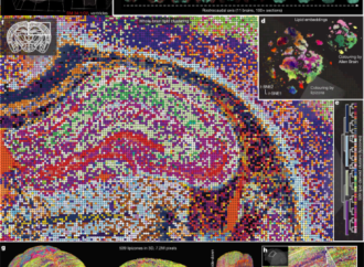
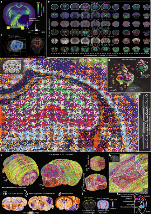
Raw MALDI–MSI data (.raw/.udp) were first converted to imzML format using RAW2IMZML (v.1.0r47). We used uMAIA¹⁵ (github.com/lamanno-epfl/uMAIA/) with default settings to process all raw data collectively (peak calling, peak matching, feature normalization), including two complete individual male brains (73 sections), male and female control sections from three individuals each (29 sections) and brains of three pregnant mice (18 sections). We identified 26,874 features initially. Quality control restricted the feature space to [M + 0] isotopologues, biological compounds (greater intensity within tissue than matrix) and features present in at least four consecutive sections. Before normalization, we reduced the feature space by removing peaks not annotated in any database, peaks with Moran’s I < 0.4, and redundant adducts. For redundant adducts mapping to the same lipid, we kept the peak with the least dropout and the highest total signal after confirming a high correlation between different adducts on non-dropout sections. This procedure yielded 1,400 m/z peaks for normalization with uMAIA.

Data preparation and feature selection

We extracted uMAIA-normalized m/z peak values for all pixels and acquisitions, transformed them back to linear scale, and stored them in a dataframe with spatial coordinates and ABA metadata (anatomical regions, colours and contours). We refined tissue masks using CCF borders, removing pixels mapping outside the brain volume. To completely remove features (m/z peaks) with residual batch effects, we performed the following feature selection procedure. We computed three scores: (1) difference between intra- and inter-acquisition variance, (2) spatial autocorrelation computed as Moran’s I (squidpy⁶⁷) and (3) number of sections the lipid measurement dropped out. First, we removed features with dropout of more than four sections (retaining 247 of 1,400 features), then we clustered lipids in the space of these scores (standardized) with kMeans (k = 10), and removed the features belonging to five out of ten clusters, corresponding to visibly corrupted distributions across acquisitions, retaining 105 of 247 features. Further technical explanations of computational methods used in this study can be found in Supplementary Methods.

Dimensionality reduction and batch integration

All differential testing and downstream analyses of the manuscript were performed directly on the uMAIA output. The dimensionality reduction and harmonization described below was used solely for clustering where strong coembedding is desired.

Dimensionality reduction was performed fitting NMF on brain 1, providing interpretable ‘global’ embeddings.

NMF seeks two low-rank non-negative matrices,

and

whose product approximates the original non-negative data matrix

Here m is the number of pixels, n is the number of lipids and k is the number of NMF factors. The number of NMF factors was selected as the number of lipid Leiden clusters maximizing the score:

where Q is the modularity, which quantifies the strength of division of a network into clusters, C the number of clusters and α a tunable parameter that controls the relative influence of modularity versus having a large number of clusters (default = 0.7). This yielded 16 lipid Leiden clusters, that is, 16 NMF factors. The NMF component matrix (left-hand side, W matrix) was seeded⁶⁸ with the lipid closest to the centroid for each cluster of lipids and the coefficient matrix with the zero-clipped cosine similarity between each lipid and the central one. We verified embedding robustness to random feature downsampling. Once the W and H matrices were learnt from brain 1, the H matrix was kept fixed and the W matrices were determined for the other brains; Harmony¹⁸ was applied on the W matrices. We also produced a low-rank, batch effect-corrected dataset by multiplying the component with the coefficient matrix. This was used for the local embedding recomputation during the clustering procedure described below. The coefficient matrix was z-standardized.

Top-down binary splitting algorithm and label transfer

We implemented a top-down hierarchical binary splitter. The algorithm splits the set of input pixels in two recursively. To perform each of the split balancing local and global variations, the globally computed W matrix (NMF coefficients for each pixel) is concatenated with the W matrix of the pixels of the parent split and of the current split, that is, the NMF is recomputed iteratively at each split. The optimal binary split is found using the backSPIN⁶⁹ approach, which is sped up by using aggregated pixel clusters instead of individual pixels (k = 60 clusters using kMeans).

A stop condition is implemented so that the splitting is halted if one of the following conditions is not satisfied: (1) differentially expressed features (inspired by Yao and colleagues⁴); (2) minimal size of clusters; or (3) coherence between consecutive sections. For differential expression, two-sided Mann–Whitney U test with BH-FDR-correction required at least 2 of 105 differential peaks at 0.2 absolute fold change and an adjusted P value of 0.05. The minimal size of a cluster was set to 200 pixels. For coherence between consecutive sections, we impose that each cluster must span at least two consecutive or four total acquisitions.

To make the split robust (that is, not instance-dependent) and to allow accurate label transfer of new datasets, at each split we trained an XGBoost binary classifier to perform the split from the embeddings. XGBoost classifiers (class rebalancing, 1,000 estimators, maximum depth 8, learning rate 0.02, 0.8 subsampling and colsample, and gamma 0.5) used early stopping on validation set (a set of held-out sections spanning the antero-posterior axis) accuracy. The XGBoost classifications on the training, validation and test sets were used as cluster labels. By this procedure, our clustering method inherently builds a transferrable annotation tree: a new pixel can be annotated by applying the local NMF to obtain its embeddings, followed by XGBoost classification, moving iteratively from the root to a terminal leaf (lipizone) of the binary tree.

To assess lipizone reproducibility and label transfer accuracy across brains, we compared the regional distributions of lipizones against the reference atlas using Pearson’s R.

Lipizone assessment, naming and visualization

We compared our clustering approach with Leiden clustering (resolution = 14.0) inspecting the confusion matrix. Results were qualitatively confirmed by visualizing the clusters with matching colours.

Lipizones were named on the basis of the ABA anatomical acronyms where they were found. Specifically, we calculated a reciprocal enrichment score from the confusion matrix of lipizones and ABA acronyms by element-wise multiplication of the enrichment of lipizones in acronyms and the enrichment of acronyms in lipizones. Lipizone colours were chosen to allow the visualization of several lipizones in the same view. To maximize contrast, we coloured the lipizones concatenating eight colourmaps, one for each of the eight lipizone classes, and assigned the colours based of the lipizone ‘leaves’ of the hierarchy. Contiguous leaf lipizones were distanced along the colourmap proportionally to their cosine similarity.

Feature restoration

We used XGBoost regression to impute features discarded during selection (the features for which measurement dropped out in a non-negligible number of sections). Features with Moran’s I ≥ 0.4 in at least four sections were candidates for restoration. For each feature, we selected the three best sections by Moran’s I for training and the fourth for testing. XGBoost models were trained to predict discarded features from the 16 Harmony-corrected NMF embeddings. Models yielding Pearson’s R ≥ 0.4 on held-out test sections were accepted and applied to all sections, resulting in 692 m/z peaks restored.

Lipid annotation

For an accurate annotation of m/z peaks, we integrated several reference sources: three bulk lipidomic experiments (ESI LC–MS with two different chromatographic columns, HILIC and Reverse Phase, and LC–MS/MS), METASPACE annotations (using the Human Metabolome Database), the LIPIDMAPS database and two published brain MS datasets (those of Fitzner and colleagues⁹ (LC–MS) and Vandenbosch and colleagues (MALDI–MSI¹¹)). We matched raw peak m/z values to reference annotations within 5 ppm, harmonizing nomenclature with goslin⁷⁰ when needed. For MALDI–MSI, we considered [M + H]⁺, [M + Na]⁺, [M + K]⁺ and [M + NH₄]⁺ adducts; for in-house LC–MS/MS, we used [M + H]⁺ and [M + NH₄]⁺ in positive mode and [M+AcO]⁻, [M − 2H]⁻ and [M − H]⁻ in negative mode.

We assigned confidence-weighted scores to each annotation: LC–MS/MS (8), ESI LC–MS (2), published studies (1), METASPACE (1 if FDR < 0.05, otherwise 0.5) and LIPIDMAPS (0, annotation transferred but unconfirmed in brain). Peak names were further prioritized using an independent quantitative LC–MS/MS dataset for sex-specific brain lipidomics (Supplementary Table 1). In cases of naming ambiguity, we prioritized lipid names covering more than 80% molar fraction among candidates; otherwise, we reported several names as the species designation. We provide detailed annotation tables (Supplementary Table 2a,b) motivating every lipid name where an overlap of an abundant and a less abundant species is possible.

We note that, in positive ion mode, a phosphatidylcholine that loses its entire choline moiety through in-source fragmentation yields an ion isobaric with the protonated phosphatidic acid of the same acyl composition; at the MS1 resolution of imaging experiments the PC in-source fragment and a genuine PA are therefore indistinguishable⁷¹. PG and PI species are detected and quantified in negative-mode LC–MS/MS in this study; we note that their negative-mode detection corroborates that the species exist in brain tissue but does not, on its own, establish that any specific positive-mode MALDI–MSI peak at a PG/PI m/z represents that species.

Peaks with annotation scores greater than four (172 nonredundant lipids) were considered unambiguous and used for the analysis in this work. The final dataset includes several lipid classes (LPC, LPE, LPA, LPS, LPG, LPI, PC, PE, PI, PS, PA, PG, SM, Cer, HexCer, Hex2Cer, TG, DG) with variable chain lengths and unsaturation degrees. As MALDI–MSI cannot distinguish isomers, we report the sum composition of carbon atoms and unsaturations, meaning an ‘individual’ lipid may comprise several isomers. The PI and PG annotations are only suggestive (based on the m/z) but should not be considered reliable in our positive ion mode MALDI–MSI data.

Data analysis and visualization methods

For visualization, we embedded our dataset in t-SNE space (perplexity 30) using z-standardized, harmonized NMF embeddings.

The 3D interpolation used radially exponentially decaying weighted neighbours with ABA regions as anatomical guides. To render, explore and film 3D maps, we used Napari⁷² and napari_animation (Supplementary Data File 1).

We assessed the residual within-cluster variability of each lipizone on brain 1 as the log determinant of the covariance matrix of that lipizone, after z-scaling lipids across the entire brain. We processed cell-type-specific bulk lipidomics data from Fitzner and colleagues⁹ using minimum–maximum normalization. For the oligodendrocyte score used in the white matter analysis, cell-type deconvolution used linear regression by non-negative least squares, with coefficients normalized to sum to 1 across cell types per lipizone. Differential lipid testing between groups used two-sided Mann–Whitney U test with BH correction (α = 0.05). A two-sided permutation test was used to evaluate lipid class enrichment.

For the similarity range score comparing the two ChP principal lipizones (ChP1–ChP2) against all other brain lipizones, for each lipizone centroid, we computed the Euclidean distances to both ChP lipizone centroids in lipidomic space restricting to differential lipids. We then expressed this as a relative distance ratio, where values below 0.5 indicated greater similarity to the first ChP lipizone and values above 0.5 to the second.

Lipid brain atlas explorer

The Lipid Brain Atlas Explorer (https://lbae-v2.epfl.ch/) is a Python-based interactive web application built using the Dash⁷³ framework for visualizing and analysing high-resolution mass spectrometry imaging data of lipids across the mouse brain.

Sample size, randomization and blinding

No statistical method was used to predetermine sample size. For the atlas backbone, two C57BL/6J male mice were densely sampled at 200-μm intervals throughout the entire brain (73 sections overall), with brain 1 used as the primary reference and brain 2 as an independent replicate to verify cluster and discovery reproducibility and label transfer performance. Sample sizes for the sex and pregnancy comparisons (n = 3 male mice, n = 3 non-pregnant female mice, and n = 3 pregnant female mice at E13.5; 29 control sections and 18 pregnancy sections) follow current conventions for comprehensive sampling in spatial transcriptomic mouse brain atlas studies. Sufficiency is supported by the successful reproduction of cluster spatial organization across all 11 brains as biological replicates (Supplementary Fig. 4d). Two additional sparsely sampled pregnant female mice were used for the PCA of pregnancy versus between-sex differences; a further four pregnant and four non-pregnant female mice were used for bulk LC–MS, two pregnant and two non-pregnant female mice were used for for snRNA-seq, and two pregnant and two non-pregnant female mice were used for immunostaining. Sections that were damaged or had low MALDI yield were excluded; these remain available as raw data on METASPACE.

The main covariates studied were sex and pregnancy, and mice were homogeneous in age. Samples were processed in a random order on MALDI–MSI; all pregnancy samples were processed after the male and female samples.

Formal blinding was not implemented in this study, in line with ARRIVE v.2.0 reporting recommendations for atlas-scale observational designs. However, different investigators performed distinct experimental stages: tissue collection and sectioning; MALDI–MSI acquisition; and downstream computational analyses. Tissue processing and acquisition used standardized protocols and predefined acquisition parameters, and downstream analyses relied on objective, quantitative lipidomic outputs generated by computational pipelines rather than on subjective scoring. Group assignments (sex, pregnancy) are intrinsic biological properties of the animals rather than experimental treatments allocated by the investigators, and are visibly apparent at the time of dissection; for the immunostaining quantification (Figs. 4n–o and 5o–p and Extended Data Fig. 11g), per-image segmentation and intensity readouts were generated by fixed Cellpose3, Spotiflow and Otsu pipelines with parameters set on a single representative sample before group identity entered any analysis.

Use of large language models

Large language models were used for code writing, manuscript drafting and editing.

Reporting summary

Further information on research design is available in the Nature Portfolio Reporting Summary linked to this article.