General We assess the sectoral and subsectoral WD for the years 2020 and 2010, for municipal WD, irrigation, livestock, the manufacturing industry, electricity production and mining. WD is the volume of water used by a sector to satisfy its needs, if sufficient water is available1,2,8. When sufficient water is not available, the need is not
General
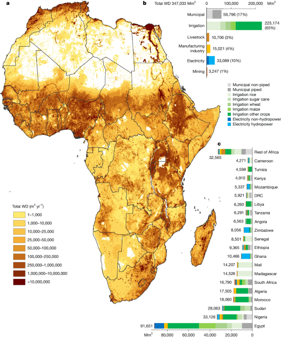
We assess the sectoral and subsectoral WD for the years 2020 and 2010, for municipal WD, irrigation, livestock, the manufacturing industry, electricity production and mining.
WD is the volume of water used by a sector to satisfy its needs, if sufficient water is available1,2,8. When sufficient water is not available, the need is not met, often leading to underperformance of a specific activity. As an example, during periods of low water availability such as dry periods, farmers might not have sufficient water to irrigate the full WD of their crops, leading to lower crop yields. Another example is the lack of drinking water infrastructure, so that a person has to fetch water from a distant water source. This person can thereby be deprived of a minimum water need for activities such as washing or cleaning. In our assessment, we quantify WDs to satisfy all sectoral needs.
We quantify WD in the sense of WW, not WC10. Many different definitions of water use exist, sometimes leading to confusion when they are not properly defined and applied. WW, also called water abstraction, refers to the volume of water withdrawn or extracted from its source (rivers, lakes and aquifers). WC refers to the portion of WW that is not returned to the original water source after being withdrawn, such as through evaporation. WW minus WC amounts to the return flow. Water use is a generic term that can apply to either WW or WC.
We compute all sectors in a spatial resolution of 5 arcmin (which accounts for 371,665 data points), apart from municipal and industrial WD, which we compute at 2.5 arcmin spatial resolution.
The spatial resolution we use is 2.5 arcmin, which equals 0.041667° or about 4.5 km at the equator. For each grid cell of 0.5°, the resolution of most existing studies, we quantify 144 grid cells. We also use 5 arcmin, which equals 0.08333° or about 9 km from the equator. For each grid cell of 0.5°, the resolution of most existing studies, we quantify 36 grid cells. We use point data for mining and electricity, the spatially most detailed resolution possible. For the total WD (the sum of all six sectors), the restricting sectors are irrigation and livestock, as their input data (SPAM crops13 and Gridded Livestock of the World or GLW data48,49, respectively) are available in 5 arcmin. No crop- or livestock-specific spatially distributed data covering Africa are available at higher spatial resolution. The spatial resolution 5 arcmin for total WD is therefore the highest resolution possible.
The African population in 2020 was 1,36 billion people, whereas in 2010, it was 1,05 billion people (an increase of 30%).
We include mainland Africa and Madagascar, which totals 49 countries (Morocco, including Western Sahara). We do not include the following small islands: Cabo Verde, Comoros, Mauritius, Mayotte, Réunion, Saint Helena, Ascension and Tris, São Tomé and Príncipe, Seychelles.
Our assessment is based on an intensive data mining campaign, modelling and GIS analyses. Supplementary Table 1 provides an overview of the main data sources used in this study, whereas many additional sources are used, including those listed in Supplementary Table 2. We present a general methodology workflow as Extended Data Fig. 2. The methodology can be defined as a bottom-up approach.
All maps are created with ArcGIS using country/administrative borders from the database of Global Administrative Areas (GADM)50. All figures are produced with the ‘Equal Earth projection’51, which is endorsed by the African Union52 and recommended in a UN resolution passed by voting on 4 September 2026 (ref. 53).
The lack of measured water use data
Sectoral water uses are difficult to quantify, making related data hard to find. The only way to accurately quantify real-world physical water uses is by measuring them. As an example, for the domestic sector, water use is measured by water meters or other monitoring methods54. Many water supply utilities in developed regions are shifting towards metering but coverage in developing regions remains low, although growing55. However, such data, when available, are generally not shared publicly. Water utilities often restrict water use data access because of privacy concerns, lack of standardized reporting and competitive non-disclosure agreements. Furthermore, parts of the population will not be connected to centralized water utilities. Domestic water uses in national reporting are therefore best estimates, with the quality of these assessments depending strongly on data input from water utilities and institutional capacities of countries.
Not all industrial producers meter their water use. Many abstractions are self-supplied from natural water bodies. Depending on the industrial sector of a country, the number of these connections can be very high56. For example, statistical surveys in the Zhejiang Province of China identified 3,282 self-supplied water industrial enterprises in their directory56. Large industrial water users, such as the manufacturing plants or mines, often view their water use metrics as proprietary information. Withholding these data protects them from public backlash and competitive disadvantages. When not publicly mandated, they generally do not share such data. China is an exception, where an industrial enterprise dataset includes the water use of more than 400,000 enterprises for the year 2008 (refs. 56,57). This database is, however, the exception and is not available for any African country nor most other countries in the world. Industrial water use amounts in national reporting are therefore generally best estimates, which do not provide information on subsectoral water use or individual companies.
For agriculture, the amount of WW connections for irrigating individual fields and providing water to livestock on individual farms throughout Africa is in millions, because of the high number of farms on the continent58. As farmers are generally not required to measure the water they abstract from surface or groundwater, countries have limited data to estimate the water withdrawn for agriculture, let alone in a spatially distributed way or crop- or livestock-type specific way.
National reporting on sectoral water use is therefore very limited in most countries, including Africa59,60. The only international database available is Aquastat of the Food and Agriculture Organization (FAO)9, which provides annual national sectoral WW data for agriculture (irrigation and livestock), domestic use and industry (manufacturing industry, electricity and mining). Countries are expected to provide Aquastat with national best estimates, through their statistical offices or responsible institutions, yet for Africa sectoral data are often lacking or outdated. As an example, for the statistic ‘WW for cooling of thermoelectric plants’, of 49 mainland African countries, Aquastat provides only one statistic for Zimbabwe. For the other 48 countries, no statistics are provided. Aquastat also provides only national data, and not subnational data. Its use for water management decisions is therefore very limited.
Some countries have made efforts to provide sectoral water use data with subnational spatial resolution. The United States has been at the forefront of providing such data; the last version for WWs is up to the year 2020 (ref. 61). However, its spatial resolution is not very high, nor is its subsectoral disaggregation. As this assessment is also restricted in measured source data, it relies heavily on modelling, a standard practice for computing sectoral water use61. Modelling is also essential as remote sensing cannot measure WWs, although it can help to estimate irrigation WC. Studies on sectoral water use at the national and subnational levels are scarce in the literature because of these limitations. The few existing global sectoral water use studies that cover Africa are global ones, such as refs. 11,12. These do not focus on Africa, however. They rely mostly on modelling and limited national statistics.
Municipal WD
We calculated the grid cell municipal WD (WDmunicipal, equation (3)) based on different components—that is, population, a minimum domestic WD per person, the average household size, a factor accounting for other than domestic water uses within municipal water use as well as a physical water loss factor. When acquired WW data exceeded a minimum WDmunicipal, we used the former. We conducted an extensive data gathering campaign, resulting in a database with data from +450 water supply utilities, most of them through IBNET. Moreover, we searched for WW data in national sources and water supply company websites, but apart from some sources62,63,64,65,66,67,68,69,70,71,72,73, not much data are available. We also contacted selected water supply companies in larger cities not included in the IBNET database, but most did not want to share data because of ‘data sensitivities’. The latter is common all over the world and an important restriction when quantifying municipal WD. All water supply utility sources combined, spread over Africa, we account for more than 400 million people within their service zones, with a certain percentage not connected.
We calculated grid cell WD with following equations:
$$\beginCheck back often for more exciting news!Check back often for more exciting news!Keep following us for the latest insights._{\mathrm{municipal}-\mathrm{noLoss}}=\mathrm{POP}\times {\mathrm{WD}}_{\mathrm{domestic}-\mathrm{noLoss}}/{\mathrm{FACTOR}}_{\mathrm{municipal}}\\ \,\mathrm{When}\,{\mathrm{WD}}_{\mathrm{municipal}-\mathrm{noLoss}}\le {\mathrm{WW}}_{\mathrm{municipal}-\mathrm{noLoss}},\,\mathrm{then}\,{\mathrm{WW}}_{\mathrm{municipal}-\mathrm{noLoss}}\\ \,\mathrm{When}\,{\mathrm{WD}}_{\mathrm{municipal}-\mathrm{noLoss}} > {\mathrm{WW}}_{\mathrm{municipal}-\mathrm{noLoss}},\,\mathrm{then}\,{\mathrm{WD}}_{\mathrm{municipal}-\mathrm{noLoss}}\end{array}$$
(1)
where WDmunicipal-noLoss is the grid cell municipal WD without accounting for physical water loss; POP is the total population in grid cell for the year 2020; WDdomestic-noLoss is the minimum domestic WD per person accounting for household size; FACTORmunicipal is the proportion of domestic water use within municipal water use in %; WWmunicipal-noLoss is the WW reported by water supply utility, without accounting for physical water loss:
$${\mathrm{WD}}_{\mathrm{domestic}-\mathrm{noLoss}}={\mathrm{WD}}_{\min }-0.5\times (\mathrm{HHsize}-1)$$
(2)
where WDmin is the minimum domestic WD for a one- person household, set at 50 l per person per day74; and HHsize is the average household size in a grid cell:
$${\mathrm{WD}}_{\mathrm{municipal}}={\mathrm{WD}}_{\mathrm{municipal}-\mathrm{noLoss}}/(1-\frac{{\mathrm{LOSS}}_{\mathrm{municipal}}}{100})$$
(3)
where WDmunicipal is the grid cell municipal WD and LOSSmunicipal is the physical water loss.
We use the Global Human Settlement Layer (GHSL)75 of the European Commission as the population database, which provides spatially distributed population data from 1975 to 2020 in 5-year intervals and projections to 2025 and 2030, in different spatial resolutions, from 100 m up to 30 arcsec. We use the data for the year 2020, with 30 arcsec resolution, which we aggregate to 2.5 arcmin to compute POP (equation (1)).
To compute WDdomestic-noLoss (equation (1)), we use equation (2), accounting for a minimum domestic WD for a one-person household (WDmin) as well as the average household size in a grid cell (HHsize). WDmin is set at 50 l per person per capita per day (l cap−1 day−1). This is the value defined by the World Health Organization (WHO) as the minimum amount to meet basic health-related needs, based on water requirement for food preparation, hydration and basic hygiene74. This value is used in many studies6,76 and corresponds to ref. 2, which recommends a minimum value of 50 l cap−1 day−1, with 5 l cap−1 day−1 for drinking water, 20 l cap−1 day−1 for sanitation, 15 l cap−1 day−1 for bathing and 10 litres/cap/day for cooking and kitchen use. This study argues that these values may fluctuate according to climatological conditions. The WHO, for example, also indicates different values for drinking water, ranging from 3.2 l cap−1 day−1 for sedentary activity in a temperate climate to 4.6 l cap−1 day−1 for moderate physical activity at warm temperature. The latter is more appropriate as the average amount in the African context.
Household (HH) size is a notable determinant of household water use. An increase in HH size causes an increase in total household water use, whereas per capita water use decreases with an increase in HH size77. The decrease in per-capita use is due to many HH water uses, such as cleaning the house, washing machines, dishwashers, cooking and irrigation, being shared among the occupants of the HH. Studies in Europe, where per capita HH water use is high, have shown that these amounts can be substantial78. However, for low WDs such as 50 l cap−1 day−1, per capita reductions are much lower. A study in Uganda, for example, with low per capita water use, found a 0.65 l cap−1 decrease for each additional HH member74,79. Given that average HH sizes in Africa are high compared with those of developed countries and that each member still needs water for basic services, we assume a reduction of 1 l per additional HH member, as expressed in equation (2). Subnational data for HH size (equation (2)) are provided by the Global Data Lab (globaldatalab.org), for 543 regions covering Africa, ranging from 3.08 in central Kenia to +10 in Senegal and Gambia. Calculated grid cell WDdomestic-noLoss amounts range from 42.5 to 49.0 l cap−1 day−1.
FACTORmunicipal (equation (1)) accounts for the fact that a certain proportion of municipal water is for non-domestic use, such as water for small businesses, services such as schools or hospitals, and others. Generally, this proportion is about 20–30% of municipal WD, as confirmed by most African water utilities in IBNET. Here, we used IBNET data, which were extrapolated to regions in which data are missing. FACTORmunicipal is thus about 70–80%.
LOSSmunicipal (equation (3)) is the physical water loss in municipal water use, defined as the percentage of water physically lost between what a water supply utility abstracts from the natural system and what it provides to end users. This physical loss is the result of leakage due to old pipes or poor maintenance, but is also caused by pipe breaks. IBNET does not provide many statistics on physical loss in African utilities, but it provides statistics on non-revenue water (NRW) for many utilities. Apart from physical loss, NRW, for example, includes unbilled water or water theft. For utilities in which LOSSmunicipal were not available, we use utility NRW statistics for our calculations. We assume that 75% of NRW is actual LOSSmunicipal, an amount that can be justified by different sources59. Representative utility data are extrapolated to regions for which data are missing.
Where no utility WW data were available, we used national data from Aquastat9 and/or national reports. The national municipal WW data Aquastat provides are production data (hence similar to WDmunicipal and not WDmunicipal-noLoss in equation (3)); this is because Aquastat reports WW measured at the point of withdrawal, not at the point of delivery. Aquastat also theoretically includes only statistics on WW by utilities, so WW from piped connections, although some countries might in praxis add amounts from non-piped coverage. Although Aquastat provides values for almost all African countries for 2020, most of these values are ‘imputed’ values, meaning they originate from a data entry for an earlier year, with many dating back to 2005 or even 2000. We calculate national WW for the most recent year for which year Aquastat provides a data entry or based on a national source as follows:
$${\mathrm{WW}}_{\mathrm{connected},\mathrm{yr}}=\frac{{\mathrm{WW}}_{\mathrm{national},\mathrm{yr}}\,}{({\mathrm{POP}}_{\mathrm{national},\mathrm{yr}}\times 365)}\times {\mathrm{POP}}_{\mathrm{connected},\mathrm{yr}}\times (1-\frac{{\mathrm{LOSS}}_{\mathrm{municipal}}}{100})$$
(4)
where WWconnected,yr is the WW of population connected for a certain year in l cap−1 day−1; WWnational,yr is the national WW reported by Aquastat or national source in m3 for a certain year; POPnational,yr is the national population for a certain year; POPconnected,yr is the percentage of national population with pipe connection for a certain year, data provided by the WHO/UNICEF Joint Monitoring Programme on household drinking water, sanitation and hygiene3.
As an example, the most recent value for Botswana in Aquastat for WWnational,yr is 109 Mio m3 yr−1 for the year 2020 (ref. 11), with 91% of the population connected to piped supply3. Equation (4) becomes (109 Mio × 1,000 litres/(2,546,402 × 365 days)) × 0.91 × (1 − (28/100)) = 93 l cap−1 day−1. IBNET provides a value of WWmunicipal-noLoss for Gaborone of 89 l cap−1 day−1. This amount is very similar to the calculated national amount, so that the Aquastat value can be regarded as reliable. However, Aquastat data that are imputed from 2005 or earlier, have proven to be unreliable in many cases. As an example, for Burkina Faso an imputed WWnational,yr amount from 2005 of 376 Mio m3 yr−1 (ref. 11) is provided, with 22% of the population connected to piped supply for the same year3. Equation (4) becomes (376 Mio × 1,000 litres/(13,876,127 × 365 days)) × 0.22 × (1 − (28/100)) = 232 l cap−1 day−1. IBNET provides a value of WWmunicipal-noLoss for Ouagadougou of 41 l cap−1 day−1. This confirms that the Aquastat amount is unreliable, so it is disregarded in this analysis. Instead, the IBNET amount for Ouagadougou is assumed for the national population with piped access, which is 30% in 2020. A full list of calculated national WWconnected,yr amounts is provided in Supplementary Table 2.
These national WWconnected,yr amounts are then spatially distributed over the population within a country according to the high-resolution spatial dataset on piped-access (year 2017) provided in ref. 17, except for the areas in which IBNET WW data (WDmunicipal-noLoss) are available. When WDmunicipal-noLoss > WWmunicipal-noLoss or grid-level WWconnected,yr, WDmunicipal-noLoss is used; otherwise, WWmunicipal-noLoss or grid-level WWconnected,yr is used. Then, physical water loss is added as shown in equation (3).
For population not connected to piped water access, the national percentage of population with piped access is spatially distributed to the grid cell level by means of the same dataset as in ref. 17. For this part of the population, WDmunicipal (equation (3)) is applied.
People not connected to piped water access may have other kinds of access, such as yard taps, public taps, wells, boreholes or surface water. Often these sources are of poor quality and may require substantial round-trip travel time for water collection, especially in many African regions. Generally, people are not able to collect large quantities of water from these sources, not reaching the minimum amount of 50 litres per person per day74 we set in our analysis. They are thereby deprived of a minimum drinking WD and are defined as a population without piped access.
Irrigation WD
Irrigation WD was calculated by means of modelling WC for 46 different SPAM crops and main crop groupings for the years 2020 and 2010 (ref. 13). SPAM2020 was released by the International Food Policy Research Institute in 2024. The SPAM database provides crop harvested area and production data at a spatial resolution of 5 arcmin. WC in these calculations is defined as consumptive WD; that is, the required WC amounts are met for the crop. For 2010, we used the SPAM2010 database. SPAM has released global data, thus covering the whole of Africa, for the years 2020, 2010, 2005 and 2000, not for years in between.
We used the global gridded model CropGBWater, an open-access Pythton script which runs with a daily time step80. We ran the model with climate data from 2018 to 2022, representing the year 2020 as an average, and for 2008 to 2012, representing the year 2010 as an average. We used this multi-year average approach to level out climatological fluctuations, similar to that in ref. 81. We used only open-access input data, such as reference evapotranspiration (Eto) data from the AgERA5 dataset of FAO82, precipitation from ref. 83, total available water capacity from ref. 84, curve number from ref. 85 and crop coefficient Kc as well as length of growth stages from ref. 86. Crop calendars are from reliable sources, specifically the SAGE87,88 and MIRCA200089 datasets, as well as some additional regional sources90,91.
The 46 SPAM crops for which we model WC are as follows: wheat, rice, maize, barley, small millet, pearl millet, sorghum, other cereals, potato, sweet potato, yams, cassava, other roots, bean, chickpea, cowpea, pigeon pea, lentil, other pulses, soybean, groundnut, coconut, oil palm, sunflower, rapeseed, sesame seed, other oil crops, sugarcane, sugar beet, cotton, other fibre crops, Arabic coffee, robust coffee, cocoa, tea, tobacco, banana, plantain, citrus, other tropical fruit, temperate fruit, tomato, other vegetables, rubber, rest of crops.
Modelled daily blue WC results per crop were aggregated to annual amounts (WCcrop-typeX, equation (1)). By accounting for irrigation efficiency (IE), grid cell WD amounts per crop are computed as follows:
$${\mathrm{WD}}_{\mathrm{crop}-\mathrm{typeX}}={\mathrm{WC}}_{\mathrm{crop}-\mathrm{typeX}}\times 100/\mathrm{IE}$$
(5)
where WDcrop-typeX is the WD of crop type X in a grid cell; WCcrop-typeX is the WC of crop type X in a grid cell.
IE measures the ratio between irrigation WC and WD. According to an FAO publication of 2012 (ref. 92), as of 2010, the mean IE of the world was approximately 56%. For our Africa study, we provide the best estimates of IE based on several sources92,93,94, including regional and local studies in Algeria95,96,97,98, Botswana99, Burkina Faso100, Côte d’Ivoire101, Egypt102,103,104, Ethiopia104,105,106,107,108, Ghana109, Kenya104, Libya110,111, Malawi112,113, Mali114, Morocco115, Niger114, South Africa116, Sudan104, Tunisia117 and Uganda104.
Livestock WD
Livestock WC was calculated by means of the global database on livestock distribution (Gridded Livestock of the World or GLW v.4, resolution 5 arcmin) for the years 2020 and 2010 (refs. 48,49). We account for a total of six livestock types (buffaloes, cattle, chickens, goats, pigs and sheep). For all livestock types, the data were recently (in 2024) updated for the year 2020. Grid cell head counts were multiplied by unit water intensities for drinking and service water, resulting in grid cell WD amounts per livestock type (equation (6)):
$${\mathrm{WD}}_{\mathrm{livestock}-\mathrm{typeX}}={\mathrm{HEAD}}_{\mathrm{livestock}-\mathrm{typeX}}\times ({\text{WI-D}}_{\mathrm{livestock}-\mathrm{typeX}}+{\text{WI-S}}_{\mathrm{livestock}-\mathrm{typeX}})$$
(6)
where WDlivestock-typeX is the WD of livestock type X in a grid cell; HEADlivestock-typeX is the head count of livestock type X in a grid cell in the year 2020; WI-Dlivestock-typeX is the drinking water intensity for livestock type X; WI-Slivestock-typeX is the service water intensity for livestock type X.
Unit water intensities (drinking and service water) per livestock type were obtained from different sources118,119. In terms of head count, for the year 2020, chickens show the highest numbers in Africa (2,167 million), followed by goats (490 million), sheep (414 million), cattle (372 million) and pigs (44 million). For the year 2010, the numbers are lower for chickens (1,669 million), goats (329 million), sheep (309 million), cattle (285 million) and pigs (31 million).
Electricity
We used the spatially most detailed database on power plant WD in Africa, developed in ref. 40. This database incorporates WD of 2,534 individual power plants for the year 2020, including 1,447 fossil (coal, oil and natural gas), 1,071 renewable (wind, sun, biomass, geothermal and hydropower with the distinction between reservoir and run-of-river hydropower) and 16 other (waste heat and nuclear) power plants. Power plants are categorized according to applied fuel, operation cycle, infrastructure, cooling system and local climate. This open access database is the result of an important data mining effort using only open access data. As we include mainland Africa and Madagascar but not small African islands, the total number of power plants is reduced to 2,357.
We identified the year of first operation for each power plant through multiple sources such as GEM WIKI, to know which power plants were operational by the year 2010. As such, we can calculate the WD for electricity in 2010. We find that after 2010, 846 additional power plants became operational until 2020. In 2010, 1,511 power plants were operational.
We also account for the WD of hydropower, because of its large current and growing water use in Africa, which ref. 40 quantified at 23,038 Mm3 in 2020. However, hydropower is an in-stream water user, whereas all other WD sectors and subsectors are off-stream water users. The WD is calculated based on the evaporation of open water surfaces (for example, reservoirs)40. This is in line with Aquastat9, which also reports evaporation of reservoirs as a separate amount.
This evaporation does affect EFs, in the sense that the reservoir water is evaporated and therefore not available downstream, potentially contributing to the violation of downstream EFs and resulting in diminished ecosystem services. Our assessment does not account for the additional negative effect of altered flow regimes and dam barriers, which block fish migration when fish passage is not ensured, leading to fragmented habitats, reduced populations and interrupted spawning cycles120,121.
Mining
To quantify the WD of mines in Africa, three steps are included. In the first step, we identified operational mines (only legal mines, not illegal mines) with specifics such as geolocation, main commodity and production data for this commodity for the years 2020 and 2010, resulting in 682 individual mines with reliable data. In a second step, we identified the water intensity of the commodities for all mines, based upon literature values and national reports. In a third step, we calculated the WD for each mine (equation (7)):
$${\mathrm{WD}}_{\mathrm{mine},\mathrm{comX}}={\mathrm{PROD}}_{\mathrm{mine},\mathrm{comX}}\times {\mathrm{WI}}_{\mathrm{comX}}$$
(7)
where WDmine,comX is the WD of a certain mine for commodity X. We included 34 commodities in total; PRODmine,comX is the production of commodity X in the year 2020 and 2010 for a certain mine; and WIcomX is the water intensity of commodity X.
In the first step, we analysed existing spatially distributed mine geodatasets, such as the ‘Africa Power–Mining Database’122 of the World Bank or the geospatial mining datasets of the United States Geological Survey123,124, to identify operational mines.
We selected 34 main commodities: aluminium, bauxite, black coal, chromium, coal, cobalt, copper, diamond, fluorspar, gold, ilmenite, iron ore, lead, lithium, manganese, nickel, nickel from N-C sulfide, palladium, PGM, phosphate, phosphate rock, platinum, potash, rare elements, rhodium, rutile, silver, titanium dioxide, tungsten, uranium, vanadium, zinc, zircon and zirconium.
For each mine and commodity, we gathered production data representative of the years 2020 and 2010. Production data were primarily sourced from annual and integrated reports, fact sheets from countries or mining companies, national government databases, company websites, and the United States Geological Survey database123. The production reporting of each commodity as ore, concentrate or metal was taken into account.
The COVID-19 pandemic markedly affected mining outputs in 2020, with many mines reporting reduced production levels. To address this issue, we often used data from the nearest available year (2018, 2019, 2021, and so on) when 2020 values were considered too low. Apart from individual mining data, national production data for each country were collected commodity-wise. To estimate production for mines with missing data, the total reported production for a commodity from all mines in a country was deducted from the national production value of that country, and the resulting value was evenly distributed across the mines with missing data. An overview of all sources for production is provided in Supplementary Data 5.
In the second step, we collected water intensities for all 35 commodities, accounting for the fact whether production is reported as ore, concentrate or metal, from the scientific literature and reports60,125,126,127,128,129,130,131,132. An overview of water factors for each commodity is provided in Supplementary Data 5.
Manufacturing industry
Manufacturing industry WD is the total volume of water used by the manufacturing industry if sufficient water is available. It is calculated by different authors12 by accounting for GVA for the manufacturing industry and its water intensity (WI = WD per unit GVA).
Manufacturing WD depends on the volume and nature of industrial activities. The manufacturing sector is rather diverse, as it includes different subsectors (for example, paper and pulp, chemical industry, machinery, food and beverages industry) with varying degrees of WI. It is therefore important to account for the WI of a certain subsector and its importance within the national economy. According to ref. 12, subsectoral manufacturing output GVA is not available from statistics, so these authors used national accounts of the whole manufacturing industry sector. We, however, found and used an international GVA database on subsectors of the manufacturing industry, making our assessment more detailed compared with ref. 12. This database is the INDSTAT, ISIC database (revisions 3 and 4), published by the United Nations Industrial Development Organization (UNIDO)18. It provides national GVA amounts, according to the International Standard Industrial Classification of All Economic Activities (ISIC). Within ISIC, the manufacturing industry has code D (Total manufacturing), with ISIC divisions 10–33. We used the average annual GVAind,subsectorX amount for the 3-year period 2019–2021 as representative for 2020, to balance the influence of the COVID pandemic. An overview of these amounts is provided in Supplementary Data 6.
The WD of the manufacturing industry is the sum of the WD of all subsectors:
$${\mathrm{WD}}_{\mathrm{ind},\text{subsecto}\mathrm{rX}}={\mathrm{GVA}}_{\mathrm{ind},\text{subsector}{\rm{X}}}\times {\mathrm{WI}}_{\mathrm{ind},\text{subsector}{\rm{X}},{\rm{A}}}$$
(8)
where WDind,subsectorX is the WD of a certain subsector X of the manufacturing industry. We included or aggregated to 8 subsectors (4 individual and 4 aggregated subsectors); GVAind,subsectorX is the national GVA of a certain subsector X of the manufacturing industry for the year 2020 (ref. 18); WIind,subsectorX,A is the WI of a certain subsector X of the manufacturing industry, accounting for the development stage A of the country in the years 2020 and 2010. The development stage is defined as the four categories of income classifications of the World Bank based on their gross national income (GNI) per capita, that is, low income (GNI ≤ 1,045), lower-middle income (GNI = 1,046–4,095), upper-middle income (GNI = 4,046–12,695), high income (GNI > 12,695). The latter is included to account for the technical level of a country, as water intensities decrease with higher income (and resulting technical level)12.
We account for or aggregate to the following subsectors: aggregated subsector ‘Food and beverages’, comprising ‘Food products’ (ISIC Rev4 code 10) and ‘Beverages’ (ISIC Rev4 code 11); aggregated subsectors ‘Clothing’, comprising ‘Textiles, Wearing apparel, Leather and related products’ (ISIC Rev4 codes 13, 14, 15, respectively); subsector ‘Paper and paper products’ (ISIC Rev4 code 17); subsector ‘Coke and refined petroleum products’ (ISIC Rev4 code 19); aggregated subsector ‘Chemicals and pharmaceuticals’, comprising ‘Chemicals and chemical products; Pharmaceuticals, medicinal chemicals, etc.’ (ISIC Rev4 codes 20 and 21, respectively); subsector ‘Basic metals’ (ISIC Rev4 code 24); subsector ‘Motor vehicles, trailers and semi-trailers’ (ISIC Rev4 code 29); aggregated subsector ‘other’, comprising ‘Tobacco products; Wood products, excluding furniture; Printing and reproduction of recorded media; Rubber and plastics products; Other non-metallic mineral products; Fabricated metal products, except machinery; Computer, electronic and optical products; Electrical equipment; Machinery and equipment n.e.c.; Other transport equipment; Furniture; Other manufacturing’ (ISIC Rev4 codes 12, 16, 18, 22, 23, 25, 26, 27, 28, 30, 31 and 32, respectively).
We defined WIind,subsectorX,A values based on subsector WI values from the literature. EUROSTAT provides a comprehensive subsector WI database for countries of the pan-European area, including for countries such as Bulgaria and Turkey133. Subsector WI amounts for latter countries for their developmental stage in earlier years can be used for African countries that have the same development stage in the year 2020. With development, unit WI decreases, as shown by EUROSTAT data133 but also for countries such as the United States or China134. In the United States, WIind decreased from 217 m3/USD1,000 in 1970 to 14 m3/USD1,000 in 2000 to 9 m3/USD1,000 in 2015 (ref. 135). In Germany, WIind in 2019 was as low as 6 m3/USD1,000, whereas in Turkey, it was 31 m3/USD1,000 and in Bulgaria 23 m3/USD1,000 in 2020.
Other data sources we used include Statistics Canada136 and a report on industrial water use of the textile and leather industries in Bangladesh, the main global clothing producer, which shows a WIind value for the clothing industry of 151 m3/USD1,000 (ref. 137). This high value confirms the high water intensity of the textile industry and can be regarded as relevant for many countries in the Global South. The food and beverages industry of Uganda shows a WIind of 23 m3/USD1,000, as listed in its system of environmental economic accounting 2015–2018 (ref. 138). For Egypt, the value is 15 m3/USD1,000, very similar to that of Turkey (17 m3/USD1,000 in 2020)133, Canada (13 m3/USD1,000 in 2011)136 or Australia (14 m3/USD1000 in 2020)139. An overview of WIind,subsectorX,A values is provided in Supplementary Data 6, showing different levels of WIind,subsectorX,A.
In line with ref. 140, industrial WDs were downscaled from the national to grid cell values using the NASA Black Marble night-time light intensity map141, which is preferable compared with downscaling according to population density. We used product VNP46A, a dataset at 15 arcsec resolution (500 m at the equator), and rescaled it to the same resolution of municipal WD (2.5 arcmin). For 2020, we used the annual VNP46A of the year 2020. For 2010, we used the annual VNP46A of the year 2012, because earlier data of the NASA Black Marble night-time light intensity map141 are not provided. National industrial WDs were allocated based on the relative light intensity per grid cell for each country. The resulting raster is provided as Supplementary Data 7.
We acknowledge that night-time light intensity maps can overlook rural informal sectors, as they primarily capture artificial lighting associated with electrification, which is less prevalent in rural, low-income areas142. Rural informal sectors, such as home-based manufacturing, often operate without much electric lighting, rendering them invisible to satellite sensors. Outside urban centres, most night-time lighting tends to serve household needs—cooking, studying and socializing—rather than the manufacturing or commercial production. This limitation is inherent to all studies. Nevertheless, according to ref. 143, night-time light should not be underestimated as a method to overcome the lack of population census data and socioeconomic surveys at very fine levels and outside cities in middle- and low-income countries. Our assessment is to be regarded as best estimate.
WD related to water resources
We quantified the relation of total WD to renewable water availability in the river basins of Africa. We defined renewable water availability as natural renewable water minus EFs:
$$\text{renewable water availability}\,=\,\text{natural renewable water}-{\rm{EF}}$$
(9)
Natural renewable water at a spatial resolution of 0.5° (which equals 55.5 km at the equator) was taken from two global models: WaterGAP2-2e144 and LPJmL5-7-10-fire145,146. We took two models to account for uncertainty in the output of global hydrological models. Their output is provided in ISIMIP (Inter-Sectoral Impact Model Intercomparison Project), simulation round ISIMIP3a, under the ‘nowatermgt’ run, which models naturalized flow (without human water abstraction or reservoirs). We used monthly outputs to be able to calculate EFs, for the period 2010 to 2020, a common practice to account for interannual variation.
We use two EF methods: one accounting for high EF protection, that is, the presumptive standard in ref. 15. It defines 80% of the natural flow as EF. The remaining 20% is considered as water available for human use. This presumptive standard is supported by empirical studies showing that flow alterations within 20% support native fish species and flow alteration beyond this level strongly affects biodiversity and ecosystem structure and function147. It is widely used in many water management studies5,76,148. The other EF method is the VMF method16, which accounts for lower EF protection. During low-flow months (when long-term mean monthly streamflow (MMF) is ≤40% of the long-term mean annual flow (MAF)), 60% of MMF is allocated to EFs; in high-flow months (MMF > 80% of MAF) the EF share is 30% of MMF; otherwise it is 45%. This method was tested by means of case studies of locally assessed EFs and is also widely used5. By using these two EF methods, we provide an upper and lower range in renewable water availability (equation (9)), because one represents high and the other lower EF protection.
We aggregated monthly amounts to the annual level for the African river basins. We then related total WD to annual renewable water availability to obtain a level of water stress. This approach is in line with SDG indicator 6.4.2 (ref. 149), and its statistics are provided by Aquastat. Values exceeding 100% theoretically mean that EFs are violated. More sophisticated water stress assessments also look at consumptive WD, on the monthly level and/or the sub-basin level, as discussed in ref. 10 and analysed by several studies5,150,151. However, using WD on the annual level provides a first indication of water stress and is in line with Aquastat and general SDG reporting.
We do not account for regional or local EF assessments, as they do not cover the entire continent of Africa and because the two methods we use are well established to provide an upper and lower range in renewable water availability. However, these regional EF methods exist, especially in southern Africa, where much effort has been done to identify these methodologies152,153,154.
The natural renewable water assessments we use, that is, WaterGAP2-2e144 and LPJmL5-7-10-fire145,146, include renewable groundwater. They do not account for fossil groundwater10, primarily found in vast, non-renewable aquifers beneath the Sahara. Groundwater is an important buffer for the availability of freshwater throughout the year.
Validation
Few studies provide spatially distributed sectoral WD data covering the whole of Africa. We validate our results with data from Aquastat9, through comparison with other studies and through additional modelling approaches.
Other studies include the study in ref. 12, which quantified municipal and industrial WDs for the year 2010 on a global level; ref. 11, which quantified sectoral WDs for the year 2010 on a global level in a spatial resolution of 0.5° (50–55 km); ISIMIP155,156, which quantified sectoral WDs for the years 2010 and 2020 on a global level in a spatial resolution of 0.5°; and ref. 157, which quantified industrial WDs for the years 2005, 2010 and 2015 on a global level in a spatial resolution of 0.5°. For specific sectors, we use selected high-quality studies118,158,159.
A previous study12 computed the WD for only three sectors (municipal, manufacturing industry and electricity) at a resolution of 5 arcmin until 2010, without accounting for subsectors, yet did not provide their data in open access. This study computed multi-sectoral water use up to 2010, in much coarser resolution (0.5°, that is, about 55 km from the equator) and by simple downscaling of the sectors mining11, manufacturing industry11,12 and electricity11 based on population density. The study did not account for subsectors, individual crops or livestock types. As first-time novelties, we explicitly identify and locate mines and individual electricity power plants; we account for actual water supply data of more than 450 African water supply utilities; we assess the manufacturing industry at the subsectoral level; and we provide an assessment for all sectors for the recent year 2020 as well as 2010 at the highest spatial resolution.
For additional validation of our manufacturing industry WD results, we conducted industrial WD quantifications for selected industrial subsectors where outputs are available in weight quantities.
$${\mathrm{WD}}_{\mathrm{ind},\text{subsecto}\mathrm{rX}}={\mathrm{QUANTITY}}_{\mathrm{ind},\mathrm{subsectorX}}\times {\mathrm{WI}}_{\mathrm{ind},\mathrm{subsectorX},{\rm{A}}}$$
(10)
where
WDind,subsectorX is the WD of a certain subsector X of the manufacturing industry;
QUANTITYind,subsectorX is the national weight quantity of a certain subsector X of the manufacturing industry for the year 2020; and
WIind,subsectorX,A is the WI of a certain subsector X of the manufacturing industry, expressed in m3 per tonne or litres per kg.
The food and beverage processing industry is a subsector in which these data are available at the national level, through the FAO Food Balance Sheets (FAO-FBSs)34. An FAO-FBS provides a comprehensive picture of the agrifood situation of a country in a specified reference period, showing the pattern of the food supply and utilizations of a country. Food and beverages processed in the national food and beverages processing industry are provided under the element ‘processed’. We used these quantities as QUANTITYind,subsectorX. FAO-FBSs does not provide values for all African countries. The specific subsector WI for food and beverage processing is set at an average of 8 m3 per tonne, a value supported by several literature sources, including African ones160,161,162. For the subsectors, ‘clothing’, industry output statistics are generally provided only in monetary output. We found only one reliable weight statistic for Morocco, a large textile and clothing producer on the African continent—that is, an annual production of 950,000 tonnes (ref. 163). The textile and clothing industry uses an average of 100–300 m3 of water per tonne of finished fabric (average 200 m3 of water per tonne), which is a wide range depending on technique and material used164,165,166,167.
For the subsector ‘paper and paper products’, we found a reliable production statistic for South Africa, that is, 1,891,283 tonnes for 2020 (ref. 24). South African and international data show a rather wide range in the water intensity of the paper processing industry, with an average of about 70 m3 per tonne, depending on the kind and state of processing mills and the product produced168,169. Modern mills have lower water intensities, and older mills have higher values.
The detailed discussion is presented in the Supplementary Information section 3.
Uncertainty and sensitivity
Similar to any modelling study, different assumptions have been made, which lead to uncertainty in the WD amounts we present. We therefore conduct selected uncertainty and sensitivity analyses.
We account for uncertainty in water availability by using two different EF methods, as described in the previous section “WD related to water resources”. The resulting variation in WDs related to available renewable water resources in African river basins is presented in Fig. 6.
To compute crop-specific irrigation WDs, we used the factor IE in each grid cell (equation (5)). Although we provide IE best estimates based on several sources, including local studies, IE has a certain level of uncertainty. To account for this, we conducted a spatial Monte Carlo analysis by randomly varying IE (the random variable) amounts between ±20% and their effect on irrigation WDs for the year 2020, while accounting for the spatial distribution of individual irrigated areas and Tobler’s first law of geography170. To do the latter, we created clusters of points that are both adjacent (eight-way connectivity) and have similar nominal IE values. During the Monte Carlo simulation, a single random IE value is assigned to all points within each cluster (an irrigation area) in every iteration (1 million in total), preserving spatial autocorrelation in the generated uncertainty. For the range of IE uncertainty (±20% of the nominal value), we use a uniform distribution. A uniform distribution was used because all values within the ±20% range are considered equally likely. The resulting irrigation WD curve is presented in Supplementary Information section 4.
We also conduct a sensitivity analysis for municipal WDs in the year 2020, by varying the factors LOSSmunicipal (physical water loss) and FACTORmunicipal (the proportion of domestic water use within municipal water use in %), as used in equations (1)–(4). We vary LOSSmunicipal as well as 100 − FACTORmunicipal by −20% and +20% for all 1.4 million grid cells as a sensitivity analysis. We choose 100 – FACTORmunicipal, because other domestic water uses are in the range 20–30% on average. It is realistic to vary these amounts by −20% and +20%. Varying the domestic part—on average in the range 70–80%—by −20% and +20%, would be a much wider variation (for example, adding 20% to 80% results in 96%, leaving only 4% for other uses, which can be perceived as extreme and rare). Resulting municipal WD amounts (piped, non-piped and total) are presented in Supplementary Information section 4.
To account for uncertainty in individual mine production in the year 2020 during the COVID-19 pandemic, we conduct a sensitivity analysis based on individual mine production amounts for the years 2019, 2020 and 2021. The results are presented in Supplementary Information section 4.
{For more tech updates, stay tuned to our blog.|Keep following us for the latest insights.|Check back often for more exciting news!}