Training of snTIMs

PsychAD cohort

Molecular profiling efforts of the PsychAD consortium include snRNA-seq from more than 6 million nuclei from the DLPFC of 1,494 unique donors¹⁵. As described in the Capstone paper¹¹, we utilized quadratic discriminant analysis using the 1000 Genomes Project^58,59 reference to divide the full cohort into five discrete superpopulations based on ancestry: EUR, AFR, AMR, East Asian and South Asian. Of these, 1,359 genotyped individuals (920 EUR, 321 AFR and 118 AMR)¹¹ had undergone snRNA-seq-based profiling; East Asian and South Asian were excluded from TIM building due to lack of sufficient power. Furthermore, PsychAD is composed of three ‘subcohorts’ (Mount Sinai National Institute of Health Neurobiobank, National Institute of Mental Health Intramural research program Human Brain Collection Core and Rush Alzheimer’s Disease Center (RADC)), of which RADC is predominantly AFR (Supplementary Table 41). We utilized snRNA-seq data from all 8 cell-type classes, and 23 subclasses (excluding 4 subclasses that are identical to classes). Finally, we note that we utilized release 2.5 of PsychAD.

Genotype and gene expression quality control for TIM training

Generation of an ancestry-specific common variant reference list

The merged PsychAD genotype dataset consisting of PsychAD-Mount Sinai National Institute of Health Neurobiobank SNP array, CommonMind SNP array, RADC whole-genome sequencing (WGS) and Alzheimer’s Disease sequencing project WGS samples was prepared as previously described¹⁵. Towards harmonizing SNP utilization across the training (merged PsychAD genotype dataset) and target (GWAS for S-TWAS) cohorts and trans-omics for precision medicine (TOPMed)-imputed SNP arrays for the MVP), we constructed ancestry-specific common variant reference panels. First, we queried all variants in the TOPMed-imputed^60,61,62,63 MVP’s⁶⁰ genotype release 4 and retained non-ambiguous biallelic SNPs with reference SNP cluster identification annotation included in individuals from the MVP that passed the following filters (see below for variant-level and sample-level quality control): population-specific minor allele frequency (MAF) greater than or equal to 0.01 and population-specific genotype missingness less than or equal to 0.05. Consequently, ancestry-specific SNPs were retained if they also had a matched superpopulation-specific MAF greater than or equal to 0.01 in the 1000 Genomes Project to ensure SNP overlap with GWAS used in S-snTWAS analysis^58,59. The resulting ancestry-specific common variant reference list comprises approximately 4.5, 7.5 and 5.1 million SNPs in EUR, AFR and AMR, respectively.

Variant-level filtering in the training cohort (PsychAD)

Variant-level filtering on the genotypes used for the TIM training requires that all the following variant inclusion criteria were met: SNPs exist in the ancestry-specific SNP list described above, MAF ≥ 0.01, based on ancestry-specific information from the National Center for Biotechnology Information Allele Frequency Aggregator (ALFA⁶⁴; EUR: SAMN10492695; AFR: SAMN10492698; AMR: SAMN10492700), or an in-cohort MAF ≥ 0.01 when ALFA information was not available or the variant did not pass the ALFA filter, in-sample minor allele count of 5 or greater, a Hardy–Weinberg equilibrium P value of 10⁻⁶ or greater, and not falling within areas of high linkage disequilibrium, such as the major histocompatibility complex (Supplementary Table 42). Finally, missing information for SNP predictors in existing TIMs were replaced with double the in-sample MAF (representing the in-sample average genotype), rounded to the nearest integer. Overall, we replaced about 0.050% of genotypes used for EUR snTIM training, and 0.069% each in genotypes used for AFR and AMR snTIM training.

Gene expression quality control

As reported in Lee et al.¹¹ and Zeng et al.¹², dreamlet was used to create pseudobulked gene expression by summing reads from the same individual. Expression for each cell type and each individual was computed as the log₂ counts per million with a pseudocount of 0.25 after aggregating all corresponding nuclei. A precision-weighted regression model was fit for each expressed gene in each cell type using the dreamlet package⁶⁵ using covariates for age, sex, postmortem interval, mitochondrial rate, ribosomal rate and disease status. To control for varying sequencing depth among snRNA-seq libraries, Pearson residuals (that is, residuals divided by their standard errors) were computed for each expressed gene and cell type and used in downstream analysis.

We limited genes to those within our expression annotation, Ensembl 104 (refs. ^66,67). Second, for each ‘subcohort’ within PsychAD (see ‘PsychAD cohort’), we independently scaled gene expression, performed probabilistic estimation of expression residuals (PEER)⁶⁸ to identify and adjust for hidden factors driving gene expression differences, and quantile normalized the resulting residualized gene expression. We utilized fastQTL⁶⁹ to determine the number of PEER factors (ranging from 5 to 50) that yield optimal genetic signal by identifying the point at which the number of significant expression quantitative trait loci (eQTLs; FDR (Benjamini–Hochberg method²¹)-adjusted two-sided P ≤ 0.05) is closest to 95% of the maximum number of significant eQTLs found across any assessed number of PEER factors. Finally, we combined residualized gene expression across the three subcohorts, and repeated scaling, PEER factor optimization and quantile normalization of the combined cohort to reduce the impact of the batch effect (Supplementary Fig. 30).

Training of cell-type-specific PrediXcan models

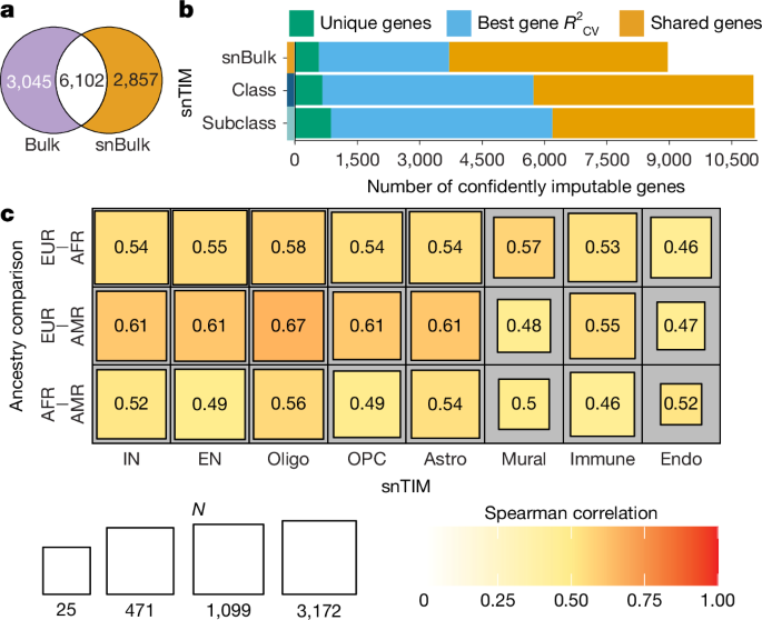
We used PrediXcan⁷ to create per-cell-type TIMs in each of three ancestries (EUR, AFR and AMR) using the quality-controlled genotypes and gene expression. Pre-processing and post-processing were done using standard scripts in R, Python 2 and Python 3. Imputable genes are considered passing R²_CV ≥ 0.01, FDR-adjusted (across cell types but within each ancestry) P_CV ≤ 0.05 and SNPs in model > 0. R²_CV and FDR-adjusted P_CV values are prediction performance R² and prediction performance P value from the ‘PredictDB’ software⁷⁰. These filtering criteria are comparable with that of other published TIMs—GTEx V8 Elastic Net models and Zeng-2024: P_CVA ≤ 0.05 (refs. ^51,71); original PrediXcan models: R²_CV > 0.01 (ref. ⁷).

To compare gene imputation models across individual TIMs or ancestries, we utilized R²_CV, a proxy of variance in gene expression explained by genetic variants serving as predictors. To compare gene imputation models across ancestries, in each pair of ancestries we selected gene–cell-type combinations confidently imputed in both ancestries, and Spearman’s correlation was performed on the resulting pairwise complete cases of confidently imputed genes.

We performed linear regression to assess the extent to which major snTIM metadata predictors (sample size and median number of nuclei contributing to the pseudobulk expression from every individual) influence snTIM performance (proxied by number of confidently imputed genes). We reported the adjusted R² as a measure of the variation explained in snTIM performance for each predictor; adjusted R² was estimated by the stats package^72,73.

We compared snTIMs against a DLPFC EpiXcan TIM¹⁶ (referred to as bulk). We compared per-gene cross-validated performance with a two-sided sign test.

GWAS phenotypes and category definitions

Traits for S-snTWAS analysis were drawn from publicly available brain disorder GWAS. To stabilize downstream analyses, inputs were date locked in 2024. At the time of publication, the PsychAD snTIMs trained in this project will be publicly released so users can freely apply these models to newer datasets.

We began with 16 traits. Four traits showed insufficient power for S-snTWAS when analysed individually, each yielding at most one FDR-significant gene and two genome-wide significant loci in their variant association results: binge-eating disorder⁷⁴, post-traumatic stress disorder (PTSD)⁷⁵, anxiety⁷⁶ and obsessive–compulsive disorder⁷⁷. We imposed a pragmatic threshold of five genome-wide significant loci to ensure robust power for S-snTWAS analysis. Our primary analyses therefore use 12 well-powered NPD and NDD GWAS summary statistics^{75,78,79,80,81,82,83,84,85,86,87,88} (Supplementary Table 12).

For targeted comparisons of I-snTWAS versus S-snTWAS (for example, Fig. 5a), we retained anxiety⁷⁶ and PTSD⁷⁵ GWAS, as both traits had adequate power for analysis in MVP (see below). For select analyses, traits were grouped as NPDs, NDDs and substance use disorders (SUDs). These groupings are analytical and not intended to mirror formal diagnostic taxonomies. We organized traits to maximize interpretability, guided by shared genetic architecture and hypothesized dominant cell type and pathway involvement. NPDs included migraines, SCZ, BD, anorexia (anorexia nervosa), insomnia, attention-deficit/hyperactivity disorder and MDD. NDDs included AD, PD, amyotrophic lateral sclerosis and multiple sclerosis. For primary analyses, we used only AUD from the SUD group; however, for category-level comparisons, SUD representation was expanded to include tobacco use disorder and cannabis use disorder.

S-TWAS using summary statistics

We utilized MungeSumstats⁸⁹ to standardize GWAS format and update reference SNP cluster identification annotations, and, where possible, we used \(Keep following us for the latest insights._Keep following us for the latest insights.=\,\fracKeep following us for the latest insights.{\frac{1}{\mathrm{cases}}+\frac{1}{\mathrm{controls}}}\) as sample size. To ensure maximum utilization of TIM SNPs, we imputed missing variants in GWAS summary statistics based on established methods⁹⁰ (Supplementary Fig. 31). Ancestry-specific imputation linkage disequilibrium panels were built on the 1000 Genomes Project with PLINK⁹¹ and the following parameters: –ld-window-kb 1000000 –ld-window 1000 –maf 0.01 –ld-window-r2 0. We used run_imputez^90,92 using a maxWindowSize of 200. To validate imputed GWAS summary statistics, we randomly sampled 1,000 SNPs per chromosome common to the GWAS and linkage disequilibrium reference panel, and correlated real and imputed z-scores (Supplementary Fig. 31). Only SNPs with a GWAS imputation R² ≥ 0.7 were retained. Finally, we performed S-TWAS for our TIMs (external data 1 (ref. ²⁰) using summary-PrediXcan (S-PrediXcan)²⁸ and Python 2. Of note, we filtered out genes located within the major histocompatibility complex, due to high linkage disequilibrium. Significant gene–cell-type combinations were determined using the FDR-adjusted two-sided P value²¹ cut-off of 0.05. The FDR-adjusted two-sided P value was calculated across all gene–cell-type combinations for each trait. Finally, we note that we did not perform GWAS imputation for tobacco use disorder and cannabis use disorder.

Enrichment for clinically relevant genes

To validate associations from the S-TWAS, we performed gene set enrichment analysis for genes with entries in the ‘neurologicCentralNervousSystem’ and ‘neurologicBehavioralPsychiatricManifestations’ columns of the Clinical Synopsis tables of the Online Mendelian Inheritance in Man database²². For our analysis, we only considered gene-specific Online Mendelian Inheritance in Man entries and not entries corresponding to large loci (for example, regions spanning multiple genes), resulting in a final set of 1,949 genes. Query TWAS genes (nominal two-sided P ≤ 0.01; only protein-coding genes) were tested for enrichment against this gene set using a one-sided Fisher’s exact test followed by FDR adjustment²¹.

Enrichment of novel genes

We qualified a GTA as novel if the association was not present in bulk DLPFC S-TWAS (FDR-adjusted two-sided P ≤  0.05 (ref. ²¹); FDR adjustment performed across all traits to mimic correction in S-snTWAS analysis) or MAGMA analysis (FDR-adjusted two-sided P ≤ 0.05; FDR adjustment performed across all traits to mimic correction in S-snTWAS analysis) performed using the MAGMA²⁴ SNP2GENE function on the Functional Mapping and Annotation of GWAS (FUMA) web portal^23,24. GWAS were prepared as above and then lifted over to GRCh37 using liftover within MungeSumstats^89,93 as required by FUMA^89,93. FUMA default parameters were used, except for the following: ‘genetype’ was set to ‘all’; the major histocompatibility complex region was custom defined to ‘28477797–33448354’ (to match the definition used in other analyses, accounting for genome build differences); window was set to 50 kb (upstream and downstream). The union (\(\cup \)) of FDR-significant S-TWAS and MAGMA hits was used to define our known list of GATs. Significant GTAs from the S-snTWAS not within this list were defined as novel. To test whether novel GTAs were enriched in snTIMs, we separated significant GTAs into two categories: significant in snBulk, and significant only in snTWAS (either class or subclass level; FDR-significant across all cellular populations). We used a two-sided Fisher’s exact test to obtain ORs and Bonferroni-corrected two-sided P values for the enrichment of novel GTAs in cell-type-specific TIMs.

TWAS fine-mapping

To address potential horizontal pleiotropic effects and account for linkage disequilibrium among SNPs utilized in snTIMs, we utilized FOCUS²⁵. FOCUS models the marginal TWAS z-scores as a multivariate Gaussian distribution given the estimated eQTL effect size and the SNP correlation and utilizes a Bayesian approach to calculate the marginal PIP for each gene, indicating its likelihood of being causal in a specific TWAS risk region. Owing to internal GWAS imputation in FOCUS, we utilized post-munging GWAS summary statistics from our pipeline before missing SNP imputation. PrediXcan-based snTIMs were converted to FOCUS-compatible format after retaining only imputable genes. FOCUS was applied both individually to each snTIM to assess effects within each cell type, and jointly (multi-cell type) for further prioritization. Unless otherwise specified, we considered TWAS-significant associations with PIP ≥ 0.5 to be fine-mapped. To quantify the proportion of S-snTWAS-significant GTAs that were fine-mapped, we summed, for each trait–snTIM combination, the number of significant GTAs with fine-mapping support and divided by the total number of significant GTAs.

We evaluated whether fine-mapped genes increase in class and subclass aggregates by assessing the total number of unique fine-mapped genes and loci in each snTIM versus the respective aggregate. Because our primary analyses utilized FOCUS applied to individual snTIMs, we repeated the analysis using multi-cell-type fine-mapping. We also applied the Wilcoxon rank-sum test to compare genes per locus in aggregates versus individual snTIMs.

To perform bi-ancestry fine-mapping for EUR and AFR I-snTWAS in MVP, we used MA-FOCUS⁹⁴. We utilized TOPMed-imputed⁶¹ genotypes in MVP so that no additional imputation was needed for SNP predictors in the snTIMs; individual-level SNP missingness was handled as above. To visualize the top AFR fine-mapped associations and their concordance with EUR fine-mapped associations and MA-FOCUS, we plotted the scaled I-snTWAS z-scores within each cell type and ancestry (for meta-analysis, we performed inverse-variance weighted meta-analysis using I-snTWAS effect size and standard error and scaled the resulting z-score). We restricted the analysis to class-level snTIMs and prioritized the top ten associations by ranking each gene by the maximum scaled AFR I-snTWAS z-score × AFR fine-mapping PIP across all considered cell-types.

mash Analysis

We implemented mash²⁶ using the mashr package in R. Owing to differences in the imputability of genes across snTIMs at the subclass level, GReX matrices are sparse; thus, we limited analysis to class-level snTIMs (Supplementary Fig. 32). Moreover, we excluded EUR classes Endo and mural, which confidently imputed a much smaller number of genes in comparison to other class-level snTIMs. Then, we performed mash on z-scores set as effect size and standard errors set to 1; we did not use the reported association effect sizes due to limitations in accurate effect size estimation in S-PrediXcan²⁸ and other TWAS methods²⁸. We filled missing values (where we do not have a model for a given gene in a given cell type), with a z-score of 0 and an arbitrarily high standard error (1 × 10¹⁰). We ran mash using data-driven covariances as recommended by the mashr authors. The mash analysis was used to obtain the probabilities of an effect (GTA) existing in a given cell type (for example, Extended Data Fig. 3a) and to assess cell-type specificity in S-snTWAS (Fig. 3a,b). For the latter, we first limited the analysis to all S-snTWAS-significant GTAs within the six cell types utilized in the mash analysis above, and further restricted GTAs to the ones having at least one but less than six (all) cell types with a significant association (local false sign rate ≤ 0.05; due to Bayesian statistics, not all S-snTWAS significant GTAs are necessarily significant in mash results).

Comparison between S-snTWAS and I-snTWAS using the same genetic data

I-snTWAS association analyses were performed as described above. For comparison, S-snTWAS association analyses were conducted using S-PrediXcan²⁸ with genome-wide variant associations derived from the same samples, binary outcomes and covariates. The resulting z-scores and effect sizes were compared with Pearson’s correlation to demonstrate the limitations of S-snTWAS in estimating accurate association effect sizes.

GTA heterogeneity analysis

I-snTWAS and snGReX-PheWAS heterogeneity statistics were calculated for S-snTWAS significant (FDR-adjusted two-sided P ≤ 0.05) GTA effect sizes in R using the metafor package⁹⁵. Heterogeneity³⁰ I²_{cell type} was calculated for genes imputable in at least two cell-type TIMs.

Targeted sn-eQTL analysis

To validate heterogeneity found in the same gene across cell types, we utilized PsychAD eQTLs calculated among EUR using multivariate multiple quantitative trait loci¹². We used the qtlPlots R package (v0.0.7) to visualize eQTLs⁹⁶. The top SNP for each cell type was extracted and linkage disequilibrium between them was examined using LDlink³¹.

TWAS pathway enrichment analysis

We used joint effect on phenotype of eQTLs associated with a gene in mixed cohorts-pathways (JEPEGMIX2-P)³² to perform linkage disequilibrium-aware competitive pathway enrichment analysis. For this analysis, we used GRCh37-aligned GWAS summary statistics (prepared as above in ‘Enrichment of novel genes’) and snTIMs converted into JEPEGMIX2-P-compatible annotation files. In addition, we incorporated biological pathways from Gene Ontology (Gene Ontology 2015), accessed through Molecular Signatures Database (MSigDB) 5.1. JEPEGMIX2-P is designed to perform pathway enrichment analysis while accounting for linkage disequilibrium structures among genetic variants. For this study, the software was enhanced to conduct competitive analyses using the correlation adjusted mean rank (CAMERA)⁹⁷ gene set test procedure, allowing for a more refined understanding of gene–pathway associations; the publicly available binary executable file was updated to include this enhancement. The derived two-sided P values were FDR-adjusted²¹ among all pathways across all ancestry-specific TIMs, and an 0.05 FDR-adjusted two-sided P value threshold was used to determine significance. To obtain more conservative estimates of the number of significant pathways per cell type while maintaining specificity, we removed all significant pathways that were ‘parents’ of other significant pathways (referred to as pathway pruning in the main text). Finally, we note that we removed the MAPT locus (defined as chromosome 17: 44928498−56807609 in GRCh38) due to the presence of haplotypes that may bias results⁹⁸. Of note, these haplotypes have been found to have a large role in AD, PD and other disorders⁹⁸.

Comparison of MG AD snTWAS with differential gene expression signatures associated with AD pathology

We utilized transcriptional profiling data from freshly isolated primary human MG, along with the corresponding AD-relevant differentially expressed gene signatures and hierarchical co-expression networks¹⁹, which were constructed using multiscale embedded gene co-expression network analysis (MEGENA)⁹⁹. The MEGENA network was constructed from FACS-sorted CD45⁺ primary human MG from 189 autopsy samples (both with and without AD-associated pathology; comprising a partially intersecting set of the FACS-MG cohort and utilizing standard settings, including: Pearson’s correlation, un-signed and minimum module size of at least ten genes. For further analyses, we retained 306 co-expression modules with 50 or more genes each, and evaluated their enrichment for differentially expressed genes and S-snTWAS signatures using the competitive gene-set test CAMERA⁹⁷ implemented in the limma R package¹⁰⁰ with default settings, using pre-ranked z-scores from the differentially expressed gene and S-snTWAS analyses. The clinical dementia rating (CDR) phenotype indicates CDR ≥ 1 versus CDR = 0, and ‘Braak’ is a categorical phenotype separating high values ≥ 5 and low values ≤ 2. β-Amyloid density indicates the mean of this metric across five measured brain regions. Functional annotation enrichment of each MEGENA module using signatures from MSigDB (v7.2)¹⁰¹ was assessed using Fisher’s exact test. The relationship between differentially expressed genes and S-snTWAS was evaluated via Pearson’s correlations between the significance estimates (signed −log₁₀(two-sided P value)) of the enrichment analyses across all modules. The modules M406, M824 and M947 were the only modules with FDR-adjusted two-sided P ≤ 0.05 in the S-snTWAS enrichments via CAMERA pre-ranked (CameraPR).

PTCA

To assess and visualize the concordance of z-scores between two datasets (for example, TWAS or summary statistics from competitive pathway enrichment analysis) at increasing significance thresholds, we performed the following analysis, which we termed PTCA. First, we scaled z-scores among all values in each dataset (using R’s base scale function, to normalize the values with a mean of 0 and a standard deviation of 1). Next, we matched identifiers (for example, trait–cell-type–gene or trait–cell-type–pathway) between the two datasets and restricted the final dataset to elements common to both datasets. Then, we performed a fixed-effect inverse-variance weighted meta-analysis using the z-scores of the dataset (standard error is assumed to be 1), and sorted the table based on the meta-analysis two-sided P value (increasing order). Finally, we measured the correlation between ordered and scaled z-scores in a step-wise restrictive manner (assuming step size = 10 and the dataset consists of 1,000 common elements, we assessed the correlation between the top 1,000 elements, followed by the top 990 elements, and so on).

Cross-disorder analysis

To compare snTWAS results across disorders, we used PTCA (described above) to assess how cross-trait z-score correlations strengthen as significance thresholds tighten, and two-sided Fisher’s exact tests to test enrichment of shared significant associations. For validation, we repeated the cross-disorder analyses with I-snTWAS in non-overlapping samples (no known overlap except for MDD) and required S-snTWAS-significant gene–cell-type associations to show concordant directions in I-snTWAS. This validation was not performed for trait pairs lacking adequate MVP power or for MDD, whose GWAS includes MVP participants. For all gene-level and pathway-level comparisons, we excluded the major histocompatibility complex and MAPT (GRCh38 chromosome 17: 44928498–56807609) regions due to haplotype complexity that can bias results (see ‘TWAS pathway enrichment analysis’)⁹⁸.

I-TWAS and snGReX-PheWAS in MVP

MVP genotype quality control

The data core team from the MVP handled genotyping, SNP imputation and initial quality control of genotypes. For this study, we utilized the MVP Release 4, which includes genotypes from 662,681 individuals. DNA was extracted from whole blood and genotyping was performed with the MVP 1.0 custom Axiom Array⁶⁰. The MVP data core called genotypes using assay for transposase-accessible chromatin (ATAC) ATAC Primer Tool (v2.11.3), Affy2vcf, PLINK⁹¹ and MVP 1.0 array library r6. Genotyping was validated using three plates of 1000 Genome samples. Rigorous genotype quality control such as plate normalization was used to improve the accuracy of genotype calling. Genotype imputation was performed using the TOPMed⁶¹ reference, SHAPEIT4 (v4.1.3)¹⁰² and Minimac4 (ref. ⁶²), and genetic principal components were generated using EIGENSOFT (v6)^103,104. We then performed sample-level and variant-level quality control on genotypes. Our quality control pipeline is based on previously established methods for other genetic analyses and optimized for maximizing input information for GReX estimation^6,74,105,106. We grouped samples by ancestry based on harmonized ancestry and race/ethnicity¹⁰⁷ (a method that integrates and harmonizes self-identified ancestry and genetic ancestry) into three ancestries (438,582 EUR, 112,346 AFR and 48,726 AMR). Using only autosomal variants, we filtered variants for MAF (0.01 or more), Hardy–Weinberg equilibrium P value (less than 1 × 10⁻⁶) and removed high disequilibrium regions (GRCh37; chromosome 6: 25500000−33500000, chromosome 8: 8135000−12000000 and chromosome 17: 40900000−45000000)¹⁰⁸. We then filtered for excess heterozygosity (four or more standard deviations from the mean), ambiguous sex (using both PLINK’s check-sex option, as well as sex chromosome aneuploidies assignments derived from plate intensity measurements) and relatedness (kinship-based inference for GWAS (KING) filter = 0.0884)^91,109. Finally, we limited variants to biallelic SNPs for individual imputation of GReX.

MVP phenotypes

Phenotypes from International Classification of Diseases-9/10 codes were transformed into phecodes using Phecode Map (v1.2)^110,111. Individuals with at least two phecodes for a given trait were considered a case for both I-snTWAS and snGReX-PheWAS analyses. Owing to the enrichment of neuropsychiatric disorders within the MVP and their high comorbidity, individuals with fewer than two phecodes were considered a control for both analyses. For the I-snTWAS analysis, only traits with at least 2% case prevalence in EUR, AFR and AMR were utilized for power considerations (Supplementary Table 12), and AD was mapped to the phecode for ‘delirium dementia and amnestic disorders’, 290, due to the way AD is routinely coded in the Veteran Affairs medical system¹¹². For the snGReX-PheWAS analysis, traits with at least 500 cases and 500 controls were considered.

GReX imputation

We estimated GReX in the MVP on an individual level using TIM-derived SNP predictor weights. Missing genotypes were replaced with double the in-sample MAF (representing the in-sample average genotype), rounded to the nearest integer.

I-snTWAS association analysis

Logistic regression analysis was performed while adjusting for sex, age and the top ten genetic principal components. Multiple test correction with FDR-adjusted two-sided P value²¹ (0.05 or less) was performed across all cell types, ancestries and traits. For comparison of I-snTWAS with S-snTWAS, we also utilized GWAS summary statistics for anxiety⁷⁶ and PTSD⁷⁵ (Fig. 4c and Supplementary Table 12).

Gene selection for snGReX-PheWAS

Owing to computational resource limitations, PheWAS analysis was performed on the top-ranked genes from the S-snTWAS and I-snTWAS. We selected significant genes from our S-snTWAS and I-snTWAS (FDR-adjusted two-sided P ≤ 0.05), and performed PheWAS on the top associations (Bonferroni-adjusted two-sided P ≤ 0.05 across all confidently imputable associations within each cell type in S-snTWAS or I-snTWAS and at least FDR-adjusted two-sided P ≤ 0.05 in the complementary snTWAS analysis; 623 unique genes) to maximize analytical yield while remaining within computational constraints. S-snTWAS genes were considered across all cell types in EUR. I-snTWAS genes were considered across all cell types and ancestries. This resulted in a total of 9,611 PheWASs (approximately 6.42% of all imputable coding gene–cell-type combinations) across 623 unique genes.

snGReX-PheWAS association analysis

As in I-snTWAS, logistic regression analysis was performed while adjusting for sex, age and the top ten genetic principal components. FDR-adjustment was performed across all considered phecodes, 623 selected genes, 3 ancestries and all cell types for considered genes. Associations with FDR-adjusted two-sided P ≤ 0.05 (ref. ²¹) were considered significant.

snGReX-PheWAS clustering

To explore the pleiotropic effects on multiple phenotypes of the top snTWAS GTAs, we performed clustering of snGReX-PheWAS results. For interpretation of associations between brain disorders, we limited phenotype categories to ‘mental disorders’ and ‘neurological’. FDR adjustment was performed across all phecodes in these categories, as well as across all 623 PheWAS genes (in all cell types and ancestries) as typical. For every trait, we extracted the top 20 S-snTWAS and I-snTWAS significant genes (FDR-adjusted two-sided P ≤ 0.05 (ref. ²¹)) in association with the target phecode (Supplementary Table 12). We extracted only the top associated gene–cell-type combination for each gene to prevent clustering due to homogeneity of GReX across cell types. We then extracted up to the top 20 phecodes significantly associated (FDR-adjusted two-sided P ≤ 0.05 (ref. ²¹)) with these gene–cell-type combinations. Ward’s hierarchical agglomerative clustering¹¹³ was performed on the association z-scores with an implementation that preserves Ward’s criterion¹¹⁴ (ward.D2 method in R). Finally, we note that we removed the MAPT locus (defined as chromosome 17: 44928498−56807609 in GRCh38) due to the presence of haplotypes that may bias results (see ‘TWAS pathway enrichment analysis’)⁹⁸.

Abundance analysis of imputable genes

We hypothesized that genes uniquely identified by snBulk versus other snTIMs were lower in abundance. To investigate this, we subsetted imputable genes into those uniquely identified by snBulk (571) and those identified by at least one other snTIM (8,388). We calculated the mean number of transcripts for every gene among all EUR individuals with available expression data for the gene. To establish the statistical significance of the difference in mean transcript count, we used the Wilcoxon rank-sum test.

Out-of-sample validation of PsychAD snTIMs

Validation of class-level PsychAD snTIMs in ROSMAP

We performed external validation of EUR snTIMs using WGS and snRNA-seq from 396 ROSMAP¹⁷ participants of EUR. WGS aligned to GRCh37 was lifted over to GRCh38 (ref. ⁹³). To determine sample ancestry, the ROSMAP genotypes underwent standard genome-wide quality control procedures^115,116. We performed an initial round of variant quality control by removing variants with less than 0.95 call rate, to avoid biases in our sample quality control. Then, we proceeded with the removal of samples that fit any of the following criteria: call rate < 0.98, absolute value of the inbreeding coefficient < 0.2, genomic sex discrepancy with reported sex and formation of pairs with relatedness (PLINK’s \(\hat{\pi }\) calculated via identity by descent) > 0.1875 (ref. ⁹¹). We applied variant quality control, excluding markers with call rate < 0.98, and Hardy–Weinberg equilibrium P < 10⁻⁶. For ancestry validation and assignment, the resulting dataset was subsequently merged with the 1000 Genomes Project reference panel, keeping variants with MAF > 0.01 and pruned with a window size of 100, a step size of 5 and a pairwise R² threshold of 0.1. The samples were subsequently projected onto the eigenvectors computed on the 1000 Genomes Project samples using EIGENSOFT’s smartpca¹⁰³. Finally, we utilized quadratic discriminant analysis-determined EUR ROSMAP samples to impute individual-level GReX using PsychAD snTIMs (the ROSMAP WGS covered 99.7% of SNPs used by the PsychAD snTIMs).

Cells from the ROSMAP snRNA-seq dataset were annotated using the PsychAD taxonomy. We first subsampled 1 million cells from both the PsychAD and the ROSMAP snRNA-seq datasets, and then used the mapping between the two datasets to infer the labels for the full dataset. We used single-cell annotation using variational inference¹¹⁷ to perform reference-based label transfer. After subsetting the genes shared between two datasets, we used the scvi-tools package¹¹⁸ to train the scVI model based on the reference dataset and inferred cell-type labels (for example, class and subclass) on the query dataset. Models were run with 5 hidden layers and 10 latent variables, and the single-cell annotation using variational inference model was trained for 20 epochs with a minimal sample of 100 cells per cluster per epoch. Last, a transfer model was trained for 100 epochs and applied to query data to assign labels based on those the model was trained on from the reference. Label transfer achieved 91.6% accuracy when evaluated using true labels from the reference dataset. ROSMAP pseudobulk data were processed identically to PsychAD.

snRNA-seq profiles were clustered according to the PsychAD taxonomy and pseudobulked per cell type. Gene expression quality control matched the PsychAD pipeline above, and pseudobulk expression was PEER residualized. For each gene–cell-type combination present in both datasets, we computed the Pearson’s correlation across individuals between observed expression and GReX, defining out-of-sample R² as r². Agreement with internal cross-validated performance was assessed by Spearman’s correlation of out-of-sample R² versus R²_CV.

Validation of PsychAD subclass-MG in FACS-MG

To perform out-of-sample validation in FACS-MG, individual genotypes (filtering detailed in ‘S-snTWAS validation’ below) were leveraged to calculate GReX using the PsychAD EUR subclass-MG snTIM. GReX was then compared with PEER-residualized FACS-MG RNA-seq (see ‘S-snTWAS validation’ below). For each gene present in both datasets, we computed the Pearson’s correlation across individuals between observed expression and GReX, defining out-of-sample R² as r². Agreement with internal cross-validated performance was assessed by Spearman’s correlation of out-of-sample R² versus R²_CV.

S-snTWAS validation

We validated S-snTWAS associations using two external datasets: FACS-MG and Zeng-2024 (ref. ⁵¹). To prepare the FACS-MG TIM, we utilized similar protocols to the PsychAD snTIMs. FACS-MG cohort samples were derived from one of three different sub-cohort (based on the site of sample preparation). Genotypes were TOPMed-imputed and a EUR SNP reference panel similar to that used for PsychAD snTIM creation was used to initially select SNPs. The 1000 Genomes Project overlap was not implemented for the reference panel used in FACS-MG TIM creation due to the application of the TIM to a single GWAS: SNP utilization for the FACS-MG AD S-TWAS was more than 95%. Samples were filtered for missingness (0.01 or less) and relatedness (KING filter = 0.0884). To perform population stratification, variants were filtered for MAF (0.05 or more), missingness (0.01 or less) and Hardy–Weinberg equilibrium P value (less than 10⁻¹⁰). Variants were pruned using PLINK’s ‘–indep-pairwise’ function (1000 10 0.02). Twenty principal components were calculated and principal component analysis was used to determine EUR individuals (EUR selection ellipsoid defined using three standard deviations and three principal components). After ancestry filtering, sample-level quality control was performed. Variants were filtered for missingness (0.01 or less) before sample filtering for missingness (0.01 or less). Subsequently, only autosomal variants were retained, and variants were filtered for MAF (0.05 or more) and Hardy–Weinberg equilibrium P value (less than 10⁻⁶). High linkage disequilibrium regions were then filtered out (Supplementary Table 42) before pruning using PLINK’s ‘–indep-pairwise’ function (50 5 0.02). We then filtered for excess heterozygosity (three or more standard deviations from the mean) before filtering samples for relatedness (KING filter = 0.0884). After retaining only quality-controlled EUR samples, downstream variant filtering was performed identically to PsychAD. RNA-seq was processed identically to PsychAD snRNA-seq, including the two step PEER factor optimization on the three sub-cohorts. After filtering, we retained 271 EUR individuals with genotypes and RNA-seq. Finally, the FACS-MG TIM was filtered identically to PsychAD snTIMs.

FACS-MG TWAS was compared with EUR subclass-MG snTWAS using publicly available AD GWAS⁷⁸. For comparison parity, FDR adjustment was applied to all confidently imputable coding genes (after removing the major histocompatibility complex locus) in FACS-MG and subclass-MG separately. We then used z-scores from each to compare TWAS using Pearson’s correlation.

PsychAD class-level snTIMs were compared to Zeng-2024 snTIMs (Supplementary Table 39) using the same MDD GWAS summary statistics¹¹⁹. GWAS summary statistics were imputed for missing SNPs to ensure adequate coverage of PsychAD snTIM SNPs. Zeng-2024 TWAS was publicly available, and identical snTIM filtering to PsychAD was applied (R²_CV ≥ 0.01, FDR-adjusted two-sided P_CV ≤ 0.05). For comparison parity, FDR adjustment was applied to all confidently imputable coding genes (after removing the major histocompatibility complex locus) in Zeng-2024 and PsychAD separately. We then used z-scores from each to compare TWAS using Pearson’s correlation.

Genetic correlation analysis

We performed bivariate heritability analysis using linkage disequilibrium score regression^120,121 to assess the genetic correlation between the aforementioned seven NPD, four NDD and three SUD GWAS summary statistics. The datasets were munged to match the HapMap3 SNP allelic information, and the linkage disequilibrium weights were pre-calculated on the 1000 Genomes Project EUR dataset¹²².

Statistics and reproducibility

To demonstrate reproducibility, we performed multiple independent and internal validation analyses. Here we summarize five key examples. (1) We performed out-of-sample replication of PsychAD snTIMs in the ROSMAP and FACS-MG cohorts (Supplementary Fig. 26a,c). We correlated imputed GReX with observed PEER-residualized snRNA-seq expression and found strong concordance between out-of-sample performance (R²_out) and cross-validation performance (R²_CV; Spearman’s ρ = 0.63; N = 70,156; P = 3.91 × 10^−7,844, and ρ = 0.55; N = 1,853, P = 1.67 × 10⁻¹⁴⁹, respectively). (2) We compared S-snTWAS results derived from PsychAD snTIMs with those obtained using independent transcriptomic imputation models, including previously published snTIMs⁵¹ and a MG-specific TIM derived from FACS-MG¹⁹ (Supplementary Fig. 26b,d). In both cases, we observed strong concordance (Pearson’s r_(13,760) = 0.78; P = 1.34 × 10^−2,772 and Pearson’s r₍₇₃₃₎ = 0.87; P = 1.32 × 10⁻²³¹, respectively). (3) To address potential bias in the cross-disorder analysis from sample overlap across GWAS datasets, we replicated the analysis replacing S-snTWAS data with independent MVP I-snTWAS data and evaluated sign concordance of results (Supplementary Fig. 14). Overall, 90% of cross-disorder associations (5,162 of 5,721) showed consistent direction of effect. (4) We further compared S-snTWAS with MVP EUR I-snTWAS (Fig. 5a). Although the overall Pearson correlation across all associations was modest, PTCA demonstrated strong concordance among top-ranked associations. (5) Finally, snTIM training incorporated fivefold cross-validation, consistent with the broader use of cross-validation for evaluating PrediXcan-style transcriptomic imputation models.

Reporting summary

Further information on research design is available in the Nature Portfolio Reporting Summary linked to this article.