Maintenance of mouse lines

All animal procedures were approved by the Austrian Federal Ministry of Women, Science and Research in accordance with the Austrian and European Union animal law (license number: BMWF-66.018/0007-II/3b/2012; BMWFW-66.018/0006-WF/V/3b/2017; GZ: 2020-0.579.989 and GZ: 2025-0.597.515). Experimental mice were bred and maintained according to regulations approved by the institutional animal care and use committee and institutional ethics committee and the guidelines of the preclinical facility (PCF) at ISTA. Mice with specific pathogen-free status according to FELASA recommendation⁵⁷ were bred and maintained in experimental rodent facilities (room temperature 21 ± 1 °C (mean ± s.e.m.); relative humidity 40–55%; photoperiod 12 h light:12 h dark). Food (V1126, Ssniff Spezialitaten) and tap water were available ad libitum. Mouse lines with MADM cassettes inserted on chromosome 11⁵⁸, Emx1-cre⁵⁹, Emx1-creER⁶⁰ and mTmG reporter⁶¹ have been reported previously and were used to generate experimental mice. All mouse lines were kept in a mixed C57/Bl6 and CD1 genetic background. Mice were used at an age range of 2–8 months for general breeding, 2–4 months (females) for collecting blastocysts, and at P21 for clonal analysis experiments in vivo. All efforts were made to minimize the number of animals by following the 3R principles.

Thank you for reading this post, don't forget to subscribe!

Timed breeding and superovulation for the generation of genetically defined blastocysts

MADM-11^TG/TG and MADM-11^GT/GT;Emx1^cre/+ or MADM-11^GT/GT;Emx1-creER^+/− stock mice were crossed to generate MADM-11^GT/TG;Emx1^cre/+ or MADM-11^GT/TG;Emx1-creER^+/− blastocysts, respectively. For scRNA-seq experiments (see ‘scRNA-seq’), mTmG reporter mice were crossed to Emx1^cre/+ mice to generate mTmG;Emx1^cre/+ blastocysts. Superovulation was performed according to the ISTA Preclinical Facility protocol. In brief, to synchronize the oestrous cycle and induce superovulation, 0.1 ml (5 IU) pregnant mare serum gonadotropin (PMSG; Sigma) was administered by intraperitoneal injection during the afternoon (between 16:00 and 18:00) of day −3 before ovulation. On day −1 (46–48 h after PMSG), 0.1 ml (5 IU) human chorionic gonadotropin (Sigma) was administered by intraperitoneal injection and the female immediately added to the male cage. Hormones in lyophilized powder form were resuspended in Dulbecco’s PBS (Sigma) and stored in aliquots at −20 °C until use.

Derivation and culture of mESCs

Blastocyst collection at E3.5 and derivation of mESCs from individually cultured blastocysts were performed as described previously⁶². Blastocysts were flushed from the uterine horn with M2 medium (Sigma) using a syringe, collected with a micropipette and washed with 1 ml of M2 medium. Blastocysts were cultured for up to 24 h in KSOM medium (Sigma) until expansion of the blastocoel and/or hatching was observed. Each blastocyst was transferred to a single well in a 96-well plate that was prepared with mouse embryonic fibroblasts (MEFs; Thermo Fisher Scientific) the day before at a density of 1.5 × 10⁴ cells per well. Blastocysts were cultured in KO-DMEM (Thermo Fisher Scientific) medium containing 15% knockout serum replacement (Thermo Fisher Scientific), 1 mM sodium pyruvate (Thermo Fisher Scientific), 0.1 mM non-essential animo acids (Thermo Fisher Scientific), 0.1 mM 2-mercaptoethanol (Sigma), 2 mM GlutaMAX (Thermo Fisher Scientific), 50 U ml⁻¹ penicillin/streptomycin (Thermo Fisher Scientific), 2i (1 µM PD0325901 and 3 µM CHIR99021, Sigma) and LIF (1 2 ng ml⁻¹, batch tested, Thermo Fisher Scientific). Once large outgrowth was observed (~7 days) the cells were passaged for the first time. mESCs were maintained on MEFs in medium containing ES-qualified FBS (Thermo Fisher Scientific)/LIF, with passaging every 3 days on average. mESCs were moved off MEFs 2 passages before generating organoids, and were plated on EmbryoMax 0.01% gelatin (Sigma) coated wells in medium containing FBS/LIF/2i⁶³ for a maximum of 10 passages. mESCs were routinely tested for mycoplasma using the LookOut Mycoplasma PCR Detection Kit (Sigma). Standard cell culture conditions (37 °C with 5% CO₂) were used throughout all procedures. Early passage (P3–P8) cells were frozen in liquid nitrogen cryovials in large stocks, using ES-qualified FBS with 20% DMSO as the freezing medium. Early passage stocks were used for all experiments (final passage of cells used to make organoids between P8 and P15).

Methanol fixation for karyotyping of mESC lines

Methanol fixation was performed according to instructions provided by Cell Guidance Systems’ karyotyping service. In short, cell cultures in 6-well plates were incubated with medium supplemented with 10 µg µl⁻¹ KaryoMAX colcemid solution (Thermo Fisher Scientific) for 30 min at 37 °C. Medium was removed and colonies were dissociated with 400 µl of pre-warmed 0.05% Trypsin EDTA (Thermo Fisher Scientific) for 5 min at 37 °C. Trypsin was deactivated with 800 µl of warm medium and cells were transferred to a 15 ml conical tube and centrifuged for 5 min at 200g. The supernatant was discarded and the cell pellet was broken by flicking the tube 20 times. Cells were treated with 2 ml of warm 0.075 M KCl drop by drop, followed by a further 2 ml dispensed slowly down the wall of the tube. The suspension was mixed by inversion and incubated for 15 min at 37 °C. Next, 10 drops of cold freshly prepared fixative (3 parts methanol (VWR) to 1 part acetic acid (VWR) by volume) were added, using a 1 ml Pasteur pipette. The suspension was mixed by gentle inversion. Samples were centrifuged for 5 min at 150g, the supernatant was discarded and the pellet was broken by flicking the tube 20 times. Cells were washed with 4 ml of cold fixative, added very slowly, and centrifuged for 5 min at 150g. The supernatant was discarded, pellet broken, and cells were finally resuspended in 1.5 ml fixative. Samples were shipped off to Cell Guidance Systems’ karyotyping service. Chromosome 8 and 11 abnormalities have been previously reported in mESC lines^64,65.

Metaphase spread for chromosome counts

Cells for metaphase chromosome spreads were fixed as described above. In preparation, Superfrost glass slides (Thermo Fisher Scientific) were cooled at −20 °C for 5 min. 100 µl of the fixed cell suspension was dropped, as a single drop, from 10–15 cm above the slide. The slide was air dried, and a coverslip was placed with Mowiol 4-88 (Carl Roth) and 1,4-diazabicyclooctane (Carl Roth) with DAPI (4′,6-diamidino-2-phenylindole, Thermo Fisher Scientific, 1:5,000 dilution) to stain DNA. Slides were imaged with a Plan-Apochromat 40×/1.2 water immersion objective using an inverted LSM 800 series confocal microscope (Zeiss), and images were processed using Zeiss ZEN Blue 2.3 and 2.6 software (Zeiss). Chromosomes were counted manually in the Zeiss ZEN Blue 2.6 software (Zeiss) and plotted using Graphpad Prism 10.2.2 (Dotmatics) software.

Generation of cortical organoids

mESCs were plated at high density so that colonies covered approximately half of the well area after 2 days of incubation. Medium was changed 1–2 h prior to dissociation with StemPro Accutase (Thermo Fisher Scientific) or CTS TrypLE (Thermo Fisher Scientific) for 5 min at 37 °C. Cells were counted with an automated cell counter, and were used only if >90% of cells were alive based on Trypan blue staining (Thermo Fisher Scientific). mESCs were centrifuged for 5 min at 200g, resuspended in Solution 1, and plated at a density of 3,500 cells per microwell in a 24w-Aggrewell plate (Stem Cell Technologies). Solution 1 contained G-MEM (Thermo Fisher Scientific), 10% knockout serum replacement (Thermo Fisher Scientific), 1 mM sodium pyruvate, 0.1 mM non-essential amino acids, 0.1 mM 2-mercaptoethanol, 2 mM GlutaMAX, 50 U ml⁻¹ penicillin/streptomycin and Wnt inhibitor (3 µM, IWR1, Sigma). No SMAD inhibitors were used as they were not required to direct cortical differentiation in mouse⁶⁶. Embryoid bodies were generated by D1, which were then transferred to 10 cm dishes with fresh Solution 1 and 2% growth factor-reduced Matrigel (Corning). On D5, organoids were gently pipetted to remove Matrigel and Solution 2 was added, containing DMEM/F12 (Thermo Fisher Scientific), 1% N2 supplement (Thermo Fisher Scientific), 0.1 mM non-essential amino acids, 2 mM GlutaMAX, 50 U ml⁻¹ penicillin/streptomycin, 1% chemically defined lipid concentrate (Thermo Fisher Scientific), and heparin (1 μg ml⁻¹; Sigma). On D7, organoids were transferred to 6-well plates and placed on an orbital shaker at low speed (50 rpm) to prevent organoid fusion. From D9, organoids were grown in medium containing a 50:50 mix of DMEM/F12 and Neurobasal (Thermo Fisher Scientific), 0.5% N2, 1% B27 (Thermo Fisher Scientific), 0.5 mM non-essential amino acids, 2 mM GlutaMAX, 50 U ml⁻¹ penicilin/streptomycin, 1% chemically defined lipid concentrate, and 50 μM 2-mercaptoethanol. Throughout the protocol medium was replaced as necessary every 2–3 days, and orbital shaker speed was increased after D9 (80 rpm). Fused organoids and/or organoids that failed to grow were discarded throughout the procedure. Standard cell culture conditions (37 °C with 5% CO₂) were applied throughout all procedures.

Induction of MADM clones in cortical organoids

Stock solutions of 4-hydroxytamoxifen (4-OHT, Sigma) were generated by dilution in 100% ethanol to a concentration 1,000-fold greater (20–80 µM) than the working solution. 4-OHT was titrated in order to generate ~1 clone per organoid on average, which varied per time point: a maximum of 80 nM for D8, 40 nM for D9–D12, 60 nM for D13, and 80 nM for D15. If 4-OHT treatment occurred on a day without medium change, medium was removed from wells containing organoids to be treated and placed in a tube, 4-OHT was added, and medium was added back to wells. After 24 h, medium was completely replaced and organoids were washed once with PBS. Organoids were collected at D20 for MADM clonal analysis, except for astrocyte analysis, which included collection at D25. For MADM clone analysis, each clone initiation time point included clones from 3 cell lines and 3 differentiations, except for D9, D11 and D12, which included clones from 2 cell lines and 4 differentiations. The numbers of clones per organoid per clone initiation time point were as follows: D8–D20 (109 clones/100 organoids = 1.09), D9–D20 (46 clones/49 organoids = 0.94), D10–D20 (93 clones/165 organoids = 0.56), D11–D20 (50 clones/67 organoids = 0.75), D12–D20 (61 clones/50 organoids = 1.22), D13–D20 (68 clones/133 organoids = 0.51), D15–D20 (40 clones/63 organoids = 0.63) and D8–D25 (39 clones/92 organoids = 0.42).

Induction of MADM clones in vivo

MADM clone induction in vivo was performed as described^56,58. In brief, MADM-11^GT/TG;Emx1-creER^+/− experimental mice were generated by crossing MADM-11^GT/GT;Emx1-creER^+/− with MADM-11^TG/TG mice. Timed pregnant females were administered 2 mg tamoxifen (Sigma) dissolved in corn oil (Sigma) by intraperitoneal injection at E10 to induce MADM clones. Live embryos were recovered via caesarean section at E18–E19 and fostered until P21. Both male and female specimens were used. In total, 30 MADM clones were obtained from 37 brains, averaging 0.81 clones per brain.

Tissue collection and cryosectioning

Organoids were fixed for 4 h or overnight in 4% paraformaldehyde (Sigma). Tissue collection from mice was performed according to previously described protocols⁵⁶. Mice were deeply anaesthetized with an intraperitoneal injection of ketamine/xylazine (65 mg kg⁻¹ and 13 mg kg⁻¹ body weight, respectively), and were confirmed to be unresponsive through pinching the paw. Perfusion was performed with ice-cold PBS followed by ice-cold 4% paraformaldehyde prepared in PBS using a peristatic pump (Carl Roth, 4–6 ml min⁻¹). Mouse brains were further fixed overnight in 4% paraformaldehyde, then washed with PBS. Organoids and mouse brains were cryopreserved with 30% sucrose in PBS for 1 and 2–3 days, respectively. Tissues were embedded in Tissue-Tek O.C.T. (Sakura) and stored at −20 °C or −80 °C until further use. All samples were cryosectioned using a CryoStar NX70 cryostat (Thermo Fisher Scientific). Brains were sectioned coronally (45 µm thickness) and were collected in PBS, and mounted onto glass slides in sequential order. Organoids were sectioned (40 µm thickness) and directly mounted onto Superfrost glass slides (Thermo Fisher Scientific). Mounted sections were air dried while protected from light and processed immediately for analysis (mouse tissue) or were stored at −20 ^oC until use (organoid).

Immunostaining

Cryosections mounted on glass slides were first rehydrated with PBS for 15 min at room temperature. For antibodies requiring antigen retrieval (PAX6, TBR2, CTIP2, SATB2, OCT3/4, NANOG and GFAP), samples were incubated in citrate buffer (10 mM citric acid, 0.05% Tween-20; pH 6.0) for 25 min at 85 °C. After cooling to room temperature and washing 3× with PBS, samples were incubated for 2 h at room temperature in blocking solution (0.5% Triton X-100 (Thermo Fisher Scientific) with 10% Donkey Serum (Thermo Fisher Scientific) in PBS. Primary antibodies were diluted in blocking solution, and samples were incubated for 16–72 h at 4 °C. After washing (3× 15 min) with PBS, secondary antibodies were diluted in blocking solution, and samples were incubated for 2–24 h at room temperature. After washing (3× 15 min) with PBS, cell nuclei were stained with DAPI (Thermo Fisher Scientific, 1:5,000 dilution) for 15 min. All sections were mounted using Mowiol 4-88 (Carl Roth) and 1,4-diazabicyclooctane (Carl Roth) and stored at 4 °C until image acquisition.

Antibodies

Primary antibodies and dilution factors included chicken anti-GFP (Aves, GFP1020, 1:1,000), goat anti-tdTomato (SICgen, ab8181-200, 1:1,000), rabbit anti-PAX6 (Cell Signaling, 60433S, 1:500), rat anti-TBR2 (Thermo Fisher Scientific, 14-4875-82, 1:400), rat anti-CTIP2 (ab18465, 1:400), mouse anti-SATB2 (Abcam, ab51502, 1:200), rabbit anti-NANOG (Abcam, ab80892, 1:500), mouse anti-OCT3/4 (Santa Cruz, sc5279, 1:200), rabbit anti-GFAP (DAKO, Z0334 1:1,000), rabbit anti-NEUROD2 (ab109406, 1:200) and rabbit anti-CASPASE3 (Cell Signaling, 9661S, 1:400). Secondary antibodies and dilution factors included donkey anti-chicken-Alexa488 (Jackson Immuno, 703-545-155, 1:1,000), donkey anti-goat-Alexa568 (Invitrogen, A11057, 1:1,000), donkey anti-goat-CY3 (Jackson Immuno, 705-165-147, 1:1,000), donkey anti-rat-Alexa594 (Life Technologies, A21205, 1:1,000), donkey anti-mouse-Alexa647 (Life Technologies, A32787, 1:1,000) and donkey anti-rabbit-Alexa647 (Life Technologies, A31573, 1:1,000). For MADM clones that were immunostained with GFAP (using donkey anti-rabbit-Alexa647), we used donkey anti-chicken-Alexa488 and donkey anti-goat-Alexa568 for immunostaining of MADM-labelled cells. For MADM clones that were immunostained with SATB2 (donkey anti-mouse-Alexa647) and CTIP2 (donkey anti-rat-Alexa594), we used donkey anti-chicken-Alexa488 and donkey anti-goat-CY3 for immunostaining of MADM-labelled cells.

Image acquisition and analysis of MADM clones

Before image acquisition, immunostained samples were first screened for MADM clones using an axioscope (Zeiss Axio Imager, Zeiss) coupled to a CoolLED p300 SB light source (CoolLED) and equipped with Plan-Apochromat 10×/0.45 and 20×/0.8 objectives (Zeiss). Green and red fluorescence were observed using an HC-dualband GFP/DsRed filter (F56-420, AHF). The presence of MADM-labelled cells was documented for subsequent confocal image acquisition. Organoid and mouse brain MADM clones were imaged with a Plan-Apochromat 20×/0.8 objective using an inverted LSM 800 series confocal microscope (Zeiss), and images were processed using Zeiss ZEN Blue 2.3 and 2.6 software (Zeiss). Confocal images were acquired in z-stacks and tiles with excitation lasers 405, 488, 561, and 640 nm. Five-channel imaging (DAPI, GFP, tdT, CTIP2 and SATB2) was specifically performed with a Leica Stellaris 5 series confocal microscope (Leica) and an HC PL APO 20×/0.75 CS objective, using a white light laser optimized by the software for all fluorophores (A488, CY3, A594, A647) except DAPI (excitation laser 405). Images were processed using LAS X 2.5.7.23225 (Leica) software. Images were imported into ImageJ (Fiji) where MADM-labelled cells were manually counted based on marker expression. MADM clone architecture was reconstructed by using previously published protocols²⁹. In short, proliferative clones are clones in which subclone sizes are ≥4 for both (red and green) subclones. Asymmetric neurogenic clones have one subclone with ≥4 cells and one subclone with <4 cells. Small neurogenic clones are those in which subclone sizes are ≤3 cells for both subclones.

Laminar positioning in MADM clones

Figure 3l, in vivo data. Data are based on laminar position as determined by DAPI staining (2 out of 263 MADM clones induced at E10–E12¹ and 9/106 MADM clones induced at E12)⁹, and laminar-specific immunostaining (0 out of 17 MADM clones at E10–E12)¹.

Organoid clearing, imaging and analysis

Delipidation

Organoids were fixed as described above; one modification to note was that the sucrose dehydration step was skipped. After fixation, organoids were embedded in 1.5% agarose, to provide structural support during the clearing process. The organoid clearing protocol was adapted from previously published tissue clearing methods^67,68,69. In brief, embedded organoids were first washed in a 50% solution of 1:1 CUBIC-L (10% w/v N-butyldiethanolamine, 10% w/v Triton X-100 in dH₂O):CUBIC-R1a (5% w/v N,N,N′,N′-tetrakis, 10% w/v urea, 10% w/v Triton X-100 1:200 5 M NaCl in dH₂O) in ddH₂O for up to 16 h at 37 °C, 300 rpm. Next, organoids were incubated in 100% 1:1 CUBIC-L:CUBIC-R1a twice for 2 h each time, at 37 °C, 300 rpm. Finally, organoids were washed with PBS twice for 2 h at 37 °C, 300 rpm, and once overnight at 37 °C, 300 rpm.

Immunolabelling of cleared organoids

Cleared organoids were incubated with chicken anti-GFP (Aves, GFP1020, 1:500) and goat anti-tdTomato (SICgen, ab8181-200, 1:500) in 0.2% PBST (note the higher antibody concentration for cleared organoids) overnight at 37 °C, 300 rpm. The primary incubation solution was removed and organoids were washed 3× for 1 h with PBS at 37 °C, 300 rpm. Next, organoids were incubated in donkey anti-chicken-Alexa488 (Jackson Immuno, 703-545-155, 1:1,000) and donkey anti-goat-Alexa568 (Invitrogen, A11057, 1:1,000) in 0.2% PBST overnight (note the higher antibody concentration for cleared organoids) at 37 °C, 300 rpm. The secondary incubation solution was removed and organoids were washed twice for 1 h with PBS at 37 °C, 300 rpm.

Refractive index matching

Once washed, organoids underwent a refractive index-matching step. Organoids were transferred through gradually increasing concentrations of CUBIC-R + (N) (30% nicotinamide and 45% antipyrine in dH₂O): 1 h steps of 25%, 50%, 75% and 100% CUBIC-R + (N) in dH₂O. After the last step, the 100% CUBIC-R + (N) solution was replaced and organoids were stored overnight before imaging.

Imaging and analysis of cleared organoids

Whole cleared organoids embedded in agarose were imaged with an Andor Dragonfly 505 spinning disk system using a 20× Lambda/NA 0.75/WD 1.00 mm objective and 488 and 561 nm excitation lasers. During imaging, organoids were immersed in either fresh CUBIC-R + (N) or mineral oil with a refractive index of 1.52. Nikon ND2 files were converted and stitched using IMARIS File Converter and IMARIS Stitcher, respectively.

3D Image analysis

Once files were converted and stitched, they were loaded into IMARIS v9.9.1. The surfaces of the organoid were reconstructed using the surface tool. Once reconstructed, IMARIS automatically calculated both sphericity and volume.

scRNA-seq

Generation of mTmG;Emx1
^cre/+ organoids for scRNA-seq

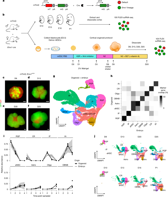
mESC lines with mTmG;Emx1^cre/+ genotype and corresponding cortical organoids were generated as described above. Two mESC lines (A and B) were used to generate two batches each (batch 1 and 2, made from consecutive passages of the same cell lines) in order to generate four replicates per time point (A1, A2, B1 and B2). Large batches were generated so that organoids could be collected at all four time points from the same batch, for each of the four batches.

Generation of mTmG;Emx1
^cre/+ embryos for scRNA-seq

Cortex samples were prepared using previously described protocols⁷⁰. In brief, embryos were collected from timed-pregnant females sacrificed by cervical dislocation whereas pups were isolated from their mothers. All embryos and pups were euthanized by decapitation. Either whole heads or extracted brains were kept in ice-cold HBSS solution. Under a dissection microscope, the cortex was carefully dissected from the brain and placed in fresh ice-cold HBSS solution. The cortex samples (or telencephalic vesicles at E10.5) were isolated free of meninges, medial and ventral structures. Isolated tissues were then pooled and processed.

Generation and fixation of single-cell suspension

To collect 10⁶ to 2 × 10⁶ fixed cells per replicate, appropriate numbers of organoids or embryos were pooled for dissociation per replicate. Embryos: A total of 40, 30, 10 and 4 brains were pooled from 8, 4, 2 and 2 litters for E10, E13, E16 and P1 time points, respectively. Organoids: D8 organoids generated from 4–5 Aggrewells, ~800 organoids; D13: ~300 organoids; D20: 80 organoids; D25: 60 organoids). Organoids or embryos were dissociated following a previously published protocol with some modifications⁷¹. Organoids or embryos were first incubated in Earle’s balanced salt solution (EBSS, Thermo Fischer Scientific) containing Papain (Worthington) and DNaseI (Worthington) for a total of 20 (D8, D13) or 25 min at 37 °C with gentle shaking at 150 rpm. Organoids or embryos were gently pipetted 3× with a P1000 tip. After adding Ovomucoid I-Albumin (Worthington), tissue suspension was briefly dissociated mechanically with a pipette. After centrifugation at 1,000 rpm for 10 min at room temperature, the cell pellet was re-suspended and further mechanically dissociated until a homogeneous cell suspension was obtained (up to 20× with a P1000 tip). The cell suspension was passed through a 70-µm filter, and centrifuged again at 1,500 rpm for 10 min at room temperature. Samples were next processed to remove debris prior to fixation. Cell pellets were re-suspended and mixed with cold Debris Removal Solution (Miltenyi Biotec). The mixture was carefully overlaid with cold PBS before centrifugation at 3,000g for 10 min at 4 °C. The top two layers containing PBS and debris were then aspirated and removed. The remaining cleaned cell suspension was collected by a last centrifugation step at 1,000g for 10 min at 4 °C. Following manual cell counting with Trypan blue, 10⁶ to 2 × 10⁶ cells were collected and pelleted. Cells were then fixed with the kit and protocol for Chromium Fixed RNA Profiling (10X Genomics, protocol CG000478, RevD). Pellets were re-suspended in a solution containing 4% formaldehyde and 1× Fix and Perm Buffer, and were stored at 4 °C for 22 h. Cells were then pelleted and re-suspended in a solution containing 1× quenching buffer. Cells were counted again, followed by addition of Enhancer solution and glycerol, after which samples were stored at −80 °C until processed.

Sample collection for MADM-CloneSeq in organoids

Organoids with MADM clones induced at D13 were collected at D20 for MADM-CloneSeq. The sample collection steps for MADM-CloneSeq were adapted from a previously published protocol⁷². Organoids were kept in cell culture membrane (Millicell) in oxygenated (95% O₂, 5% CO₂) artificial cerebrospinal fluid (ACSF) containing (in mM): 118 NaCl, 2.5 KCl, 1.25 NaH₂PO₄, 1.5 MgSO₄, 1 CaCl₂, 10 glucose, 3 myo-inositol, 30 sucrose, 30 NaHCO₃ prepared with ultra-distilled water; pH 7.4, at 35 °C, until sample collection.

All work surfaces and equipment were cleaned using RNase away solution (Thermo Fisher Scientific) prior to experiments. Single organoids were transferred to a LNscope 240XY miscroscope (Luigs & Neumann) and superfused with ACSF at a rate of 0.5 ml min⁻¹ at room temperature. Individual clones were visualized under a 20× objective and with ImageJ software. To observe red or green fluorescence, light was emitted from a LED light source (CoolLED). Glass pipettes (B150-86-10, Sutter Instrument) previously autoclaved, were pulled using a P1000 pipette puller (Sutter Instrument) to generate pipettes with an opening of around 3–5 μm. Before use, each pipette was filled with 3.5 μl of pipette solution, which consisted of RNase inhibitor (Takara, 1.95%) in RNase-free PBS (Invitrogen) filtered through a 0.22-μm filter. Red or green fluorescent neurons were approached with the pipette under positive pressure to avoid tissue contamination of the pipette tip. When contact with the cell membrane was made, tight seal formation was achieved under infrared differential interference contrast (IR/DIC) visualization. The complete aspiration of the cell body was immediately performed by applying gentle and steady suction while monitoring under fluorescence, which typically takes 5–10 s. The negative pressure was removed immediately once the target cell was collected and the pipette was carefully withdrawn from the acute slice to avoid contamination. The content of each pipette was directly transferred into individual PCR tubes and kept at −80 °C until cDNA library preparation.

Preparation of cDNA libraries and sequencing

10X Genomics: experiments were performed by the Next Generation Sequencing Facility at Vienna BioCenter Core Facilities (VBCF-NGS), member of the Vienna BioCenter (VBC), Austria. Single-cell libraries were prepared based on the 10X Genomics Flex workflow according to manufacturer’s instructions (CG000527). In order to detect GFP and tdTom mRNA expression, custom probes were designed according to 10X Genomics Technical Note CG000621 and ordered from Integrated DNA Technologies (IDT) as 4 different pools, one for each FLEX barcode sequence (BC001–BC004, custom probe sequence are provided in Supplementary Table 1). Custom probes were added to the mouse probes (PN-100496, 10X Genomics) following the manufacturer’s instructions (CG000621). MADM-CloneSeq: cDNA libraries for individual MADM-CloneSeq cells were were prepared using Smart-seq3 protocol⁷³ in 3 batches (96-well plates). Sequencing was performed at VBCF-NGS on NovaSeqX platform (Illumina).

Bioinformatic analysis

Initial analysis 10X Flex organoid data

All bioinformatic analysis was performed using a pipeline developed in-house⁷⁴. Fastq files were processed using refdata-cellranger-mm10-3.0.0 and cellranger v8.0.0 with GFP and tdTom sequences added to Chromium_Mouse_Transcriptome_Probe_Set_v1.0.1_mm10-2020-A.csv. Filtered feature matrix files (in h5 format) were used for downstream analyses in R v4.3.2 using the Seurat v5.0.1 package⁷⁵. Initial filtering for high quality cells: nFeature_RNA > 1000 & nFeature_RNA < 8000 & nCount_RNA < 40000 & percent.mt <5. We determined cell clusters using FindNeighbors (dims = 1:25) and FindClusters(resolution = 0.3). Significance of differential expression of GFP was used to determine GFP expressing cell clusters. Stressed cells were determined using granular functional filtering (Gruffi)⁷⁶. In brief, Gruffi uses gene sets from Gene Ontology (GO) pathways to calculate GO scores and identifies stressed cells by integrating multiple scores. We obtained relevant gene sets from org.Mm.eg.db (v3.18.0) using 2 terms defining stress: GO:0061621 (canonical glycolysis), GO:0034976 (response to endoplasmic reticulum stress). We found that both RGPs as well as glia cells scored high for the above terms. Therefore, we included 2 gene sets defining non-stressed cells: glia GO:0042063 (gliogenesis) and RGPs: GO:0021872 (forebrain generation of neurons), GO:0021873 (forebrain neuroblast division). Before Gruffi analysis cluster analysis was performed again: FindNeighbors (reduction = “pca”, dims = 1:30), FindClusters(resolution = 2).

Initial analysis 10X Flex mouse in vivo data

Initial filtering and identification of GFP expressing clusters of mouse in vivo data was performed as for organoid data with nCount_RNA < 20000. Clustering analysis: FindNeighbors (reduction = “pca”, dims = 1:15), FindClusters(resolution = 0.25).

Tissue origin of Emx1
⁺/Gfp
⁺ cells in organoids

Supplementary Figs. 2 and 3. This analysis was performed as for embryonic data with modifications (see below). We used the reference data prepared for the mouse in vivo analysis for label transfer: organoid D8 to reference e11.0, organoid D13 to reference e13.5, organoid D20 to reference e16.5, organoid D25 to reference e18.0. Identification of anchors and label transfer: FindTransferAnchors (normalization.method = “SCT”, reference.reduction = “pca”, dims = 1:20), TransferData (dims = 1:20). Note that during this analysis we identified that a group of D8 cells that was previously labelled as Gfp⁺ was actually Gfp-negative. To remove these cells we clustered D8 data with higher resolution, FindClusters (resolution = 0.6) and removed cluster 19 (333 cells) from downstream analyses.

Tissue origin of Emx1
⁺/Gfp
⁺ cells for mouse in vivo

Supplementary Figs. 4 and 5. Analysis of Gfp expression identified a number of cell clusters that did not express Gfp. To further investigate the origin of these cell clusters we compared our 10X FLEX scRNA-Seq data (before extraction of Gfp expressing cells) to a reference dataset that investigated multiple brain tissues during embryonic development²⁵. We obtained read counts (in loom format) and additional annotation data from http://mousebrain.org/. We compared the E10 data from this study to reference E11.0 (SampleIDs: 10×40_3, 10×40_4, 10×40_5, 10×40_6), E13 from this study to reference E13.5 (SampleID: 10×14_4), E16 from this study to reference e16.5 (SampleID: 10×17_4) and P1 from this study to reference E18.0 (SampleID: 10×32_2). Cell cycle states were assigned using marker genes for G/M and S phase (https://github.com/hbc/tinyatlas/tree/master) and the CellCycleScoring function in Seurat. We normalized, scaled data and partially regressed out cell cycle effects using SCTransform with parameter: vars.to.regress = (S.score – G2M.score), separately for reference samples and samples from this study. We transferred annotations from reference to data from this study using FindTransferAnchors (normalization.method = “SCT”, reference.reduction = “pca”, dims = 1:15) and TransferData (dims = 1:15). Note that the Class ID was obtained from http://mousebrain.org/development/celltypes.html and was assigned via the ClusterName annotation given in the loom file. The Subclass ID originates directly from the loom file annotation. In order to simplify the annotation we identified the majority Subclass label in each seurat cluster (FindNeighbors (dims = 1:25), FindClusters(resolution = 1)) and assigned cell labels accordingly. For final presentation we combined Subclass and Class IDs and focused on annotations with >3% abundance.

Data integration and cell-type annotation

Figure 1 and Extended Data Figs. 2 and 14. To allow direct comparison between organoid and embryonic data we performed data integration. To this end, we utilized cluster similarity spectrum integration (CSS)⁷⁷. CSS relies on cell clusters, identified in each sample, which it uses as an intrinsic reference for integration across samples. We merged mouse in vivo and organoid data (filtered for Gfp expressing cells as described above), joined all layers, and performed standard processing: NormalizeData, FindVariableFeatures (nfeatures = 5000), ScaleData and RunPCA (npcs = 30). Integration was performed with simspec (v0.0.0.9000) and cluster_sim_spectrum (label_tag = “group”, cluster_col = “seurat_clusters”, use_scale = F, var_genes = VariableFeatures([Seurat object])), where group defined either in vivo mouse or organoid. Cell-type identification (Fig. 1g, Extended Data Fig. 2a): dimensionality reduction was performed with RunUMAP (reduction = “css”, dims = 1:ncol(Embeddings ([Seurat object], “css”)), n.neighbors = 10, metric = “cosine”, n.components = 2, min.dist = 0.2). We defined clusters in the integrated data using FindNeighbors (reduction = “css”, dims = 1:ncol(Embeddings([Seurat object], “css”))) and FindClusters (resolution = 1). We manually associated seurat clusters to cell types using marker genes, seurat clusters, location on the UMAP and developmental timing of appearance: neurons: Neurod2, intermediate progenitors: Eomes/Top2a, RGP: Hes5/Top2a, astrocytes: Aldh1l1, oligodendrocytes: Olig2, olfactory bulb neuroblasts: Dlx5, Cajal–Retzius cells: Nhlh2, adult stem cells: mixed markers, linked to olfactory bulb neuroblasts, oligodendrocytes and astrocytes, appearing late in development. Down-sampling: owing to the use of multiple replicates, our dataset contained ~4× more organoid than embryo cells. To equalize this number for downstream analyses we down-sampled the data using SketchData (ncells = 35000, method = “LeverageScore”, sketched.assay = “sketch”). Such analysis identified 28,568 organoid cells, which we extracted and combined with the 24,942 embryonic cells. We used this down-sampled dataset for Extended Data Figs. 2 and 14, Fig. 1g–j and for marker gene analysis. Cell-type marker gene overlap was identified using FindAllMarkers (only.pos = T), separately for organoid and embryo data. We determined either the % overlap of the top 100 marker genes (Fig. 1h) or the intersection of the top 20 marker genes (Extended Data Fig. 2b) of each cell type for organoid/mouse in vivo data to prepare figures. Emx1 expression (Extended Data Fig. 2c): we determined pseudobulk expression for each cell type using AggregateExpression and plotted normalised expression. Compare cell-type abundance dynamics during development between organoid and in vivo (Fig. 1i): For this analysis we transferred the cell-type labels from the embryo data from this study to reference datasets^25,26. For²⁵ data we used data from E11.0 (SampleID: 10×40_3, 10×40_4, 10×40_5, 10×40_6), E13.5 (SampleID: 10×14_4), E16.5 (SampleID: 10×17_4) and E18.0 (SampleID: 10×32_2). We extracted cells with the following subclass annotations: Cajal-Retzius, cortical hem, cortical or hippocampal glutamatergic, dorsal forebrain, forebrain, forebrain astrocyte, forebrain glutamatergic, neuronal intermediate progenitor, glioblast, mixed region astrocytes, committed oligodendrocyte precursor, oligodendrocyte precursor cell, oligodendrocyte. For²⁶, we used data from E11 (GSM4635072), E13 (GSM4635074), E16 (GSM4635077), P1 (GSM4635080) and extracted cells with the following New_cellType annotations: apical progenitors, intermediate progenitors, immature neurons, Cajal–Retzius cells, migrating neurons, SCPN, CThPN, DL CPN, UL CPN, layer 4, NP, layer 6b, cycling glial cells, astrocytes and oligodendrocytes. For label transfer we normalized, scaled data and partially regressed out cell cycle effects using SCTransform as described before, separately for embryo data from this study and reference data^25,26. We transferred annotations using FindTransferAnchors (normalization.method = “SCT”, reference.reduction = “pca”, dims = 1:15) and TransferData (dims = 1:15). We determined relative abundances of cells for each cell type at each developmental time points for embryo data from this study, and reference datasets^25,26 and plotted the mean ± s.d. of these data points. For organoid data we plotted the mean (connected lines in the figure) as well as the actual relative abundances for the four biological replicates.

Matching in vivo mouse developmental age to organoid differentiation stage

Extended Data Figure 1e,f. We used transcriptional signature and relative abundance changes of key cell types to identify the matching embryonic age to our organoid data. (Extended Data Fig. 1e): For the heatmaps, we calculated pseudobulk expression levels of neurons and RGPs at the indicated time points for ref. ²⁵ and our organoid data by averaging normalised expression. Next, we calculated all pairwise Pearson correlations within one cell type using all genes shared between datasets. We transformed correlations to z-scores within each reference time point. For heatmap plotting, we adjusted the data matrix so that the highest z-score at each organoid time point is 0 allowing direct comparison to the best match. (Extended Data Fig. 1f): we used two published datasets^25,26. For data from ref. ²⁵, we used data from E9–E18 in one-day intervals (10 samples). We extracted cells using a stepwise approach based on annotation in the loom file. (1) We extracted cells with a forebrain region annotation. (2) From that dataset, we extracted cells with the following subclass annotations: cortical hem, cortical or hippocampal glutamatergic, dorsal forebrain, forebrain, forebrain astrocyte, forebrain glutamatergic, neuronal intermediate progenitor, committed oligodendrocyte precursor, oligodendrocyte precursor cell, oligodendrocyte. (3) From this dataset we removed cells with the following class annotations: ependymal, glioblast, Cajal-Retzius. To match cell-type annotations across references we combined all class annotations containing astrocyte or oligodendrocyte to glia and renamed neuroblast to intermediate progenitors. For ref. ²⁶, we used data from E10–E18 in one-day intervals, as well as P1 and P4 (11 samples). We extracted cells with the following New_cellType annotations: apical progenitors, intermediate progenitors, immature neurons, migrating_neurons, SCPN, CThPN, DL CPN, UL CPN, layer 4, NP, layer 6b, astrocytes, oligodendrocytes. To match cell-type annotations across references, we renamed apical progenitors to ‘radial glia’, combined astrocytes and oligodendrocytes to ‘glia’ and combined all other annotations (except for intermediate progenitors) to ‘neurons’. For organoid data, we used the annotation described above and combined astrocytes and oligodendrocytes to glia. Since we were interested in the trends of the abundance changes, we plotted reference data as a smoothed curve (method = ‘loess’, formula = ‘y ~ x’) with geom_smooth(fill = “grey70”, colour = “grey50”, level=0.9). Note that for this analysis only the metadata from the respective datasets were used, since no integration or label transfer was necessary.

MADM-CloneSeq data processing

We obtained MADM-CloneSeq data from 287 cells. Alignment was performed using STAR (v.2.7.9a)⁷⁸ on GRCm39 and Gencode vM27 with STAR parameters:–outFilterMultimapNmax 1,–outSAMstrandField intronMotif,–outFilterIntronMotifs RemoveNoncanonical,–outFilterScoreMinOverLread 0.22,–outFilterMatchNminOverLread 0.22. Note that we only used the R2 reads from paired end sequencing for this analysis. Reads in exonic and intronic regions (Gencode vM27) were counted using the aligned bam files produced by STAR and summarizeOverlaps (GenomicAlignments v1.40.0, R v4.4.0) with singleEnd=TRUE, mode = “IntersectionNotEmpty”, ignore.strand = T, inter.feature = T parameters. We combined exonic and intronic reads and used the resulting expression matrix for CreateSeuratObject (min.cells = 3, min.features = 300), to prepare a Seurat object with 279 cells. We used annotated organoid data from D20 and D25 for normalized marker sum (NMS) analysis. We identified top 200 marker genes for each cell type (aNSC, astrocyte, Cajal–Retzius cell, neuron, intermediate progenitor, OBNB, oligodendrocyte and RGP). Such analysis identified 1270 unique genes (minimum of 154 genes per group). Next, we assigned each gene to one cell type through the highest expression. We calculated (1) the mean expression of the top 154 genes (highest expression) for each cell type to determine (2) one mean expression value for each cell type in the reference. For MADM-CloneSeq, mean marker gene expression was calculated as for the reference. The final NMS score was calculated as: mean cell-type marker gene expression in MADM-CloneSeq divided by the mean cell-type marker gene expression in reference. We determined the highest NMS score for non-projection neuron cell types (non-neuron NMS). Heatmap and clustering analysis of NMS scores identified 3 clusters of PatchSeq cells with either high neuron NMS score (largest cluster, 249 cells) or high score in any other cell type (2 smaller clusters with 13 and 17 cells). We assumed that cells with a high score in a non-neuron cell type are either patched cells that were not neurons or that had a high amount of contaminating RNA from surrounding, non-neuronal cells. In both cases such cells would confound downstream analysis and were removed. We found that non neuronal cells were characterized by a ratio of neuron NMS/non-NMS of 1.2 (95th percentile: 1.195). We used a cutoff of 0.3 neuron NMS score to identify cells with a poor sequencing quality, to reduce noise. High quality neurons were defined as cells with neuron NMS / non-NMS > 1.2 and neuron NMS score > 0.3 (215 cells). Note that remaining 64 cells consisted of 31 low quality cells (highest NMS score <0.31) and 33 high quality cells (highest NMS score > 0.31). As such ~87% of high quality cells (215/248 cells) are of neuronal identity. For data integration we identified Seurat clusters in MADM-CloneSeq cells. Note that library preparation was performed in 3 batches (plates) and batch effects were considered in downstream analyses: SCTransform (vars.to.regress = c(“plate”, “NMS_Neurons”), RunPCA (assay = “SCT”), FindNeighbors (dims = 1:12), FindClusters (resolution = 2.5).

Neuron analysis

Figure 4b–h and Extended Data Figs. 12 and 13. Data integration: we prepared reference data²⁶ (E12, E13, E14, E15, E16, E17, E18_S3 and P1_S1) by extracting cells from the neuronal lineage (New_cellType annotations: Apical progenitors, Intermediate progenitors, Immature neurons, Migrating neurons, SCPN, CThPN, DL CPN, UL CPN, Layer 4, NP, Layer 6b) and processed each sample separately: NormalizeData, FindVariableFeatures(nfeatures = 3000), ScaleData, RunPCA, FindNeighbors(dims = 1:15), FindClusters(resolution = 0.8). We extracted organoid neuronal lineage cells (RGP, intermediate progenitor, neurons) from D13, D20 and D25 and processed each sample (D13, D20, D25) separately: NormalizeData, FindVariableFeatures (nfeatures = 5000), ScaleData, RunPCA (npcs = 30), FindNeighbors (dims = 1:15), FindClusters (resolution = 0.8). Finally we combined all datasets (reference, organoid, PatchSeq) and performed integration: NormalizeData, FindVariableFeatures (nfeatures = 3000), ScaleData, RunPCA (npcs = 30), cluster_sim_spectrum (spectrum_type = “corr_ztransform”, label_tag = “mergeGroup”, cluster_col = “seurat_clusters”). The mergeGroup was either developmental age (reference, organoid) or plate (MADM-CloneSeq). Reference UMAP and annotation: To prepare a common reference UMAP we extracted reference cells from the integrated data and performed dimensionality reduction in integrated (css) space: RunUMAP (reduction = “css”, dims = 1:ncol(Embeddings([Seurat object], “css”)), n.neighbors = 30, metric = “euclidean”, n.components = 3, min.dist = 0.3, return.model = T, seed.use = 2401, reduction.name = “umap_3d”). We annotated cell types using reference annotation and marker gene expression via Seurat clusters: FindNeighbors (dims = 1:150, reduction = “css”), FindClusters (resolution = 1.6). Annotating organoid data: we projected organoid cells onto the reference UMAP: ProjectUMAP(query = [organoid Seurat object], query.reduction = “css”, query.dims = 1:ncol(Embeddings([organoid Seurat object], “css”)), reference = [reference Seurat object], reference.reduction = “css”, reference.dims = 1:ncol(Embeddings([reference Seurat object], “css”)), reduction.name = “umap_3d”, reduction.model = “umap_3d”) and identified nearest reference cells for each organoid cell in 3D UMAP space using nn2 function (RANN package v2.6.1). This analysis identified the 10 closest reference cells for each organoid cell. We then identified the reference Seurat clusters of each of 10 closest reference cells and assigned the cluster name with the highest frequency. Note that for 86.5% of organoid cells >=80% of reference annotations were matching. For ~1.9% of organoid cells, no reference annotation could be assigned as 2 or more reference annotations had the same frequency. Cell-type annotation for organoid data was assigned using Seurat clusters as for the reference data. Cortical layer marker analysis (Extended Data Fig. 12a-b): we calculated DEGs between upper layer and lower layer cells using FindMarkers for reference and organoid data separately and plotted the average log₂ fold change as indicated in the figure legend. MADM-Clone-Seq analysis: we removed 2 cells with uncertain clone assignment for further analyses. We projected MADM-CloneSeq cells on the reference 3D UMAP using ProjectUMAP (query = [MADM-CloneSeq Seurat object], query.reduction = “css”, query.dims = 1:ncol(Embeddings([MADM-CloneSeq Seurat object], “css”)), reference = [reference Seurat object], reference.reduction = “css”, reference.dims = 1:ncol(Embeddings([reference Seurat object], “css”)), reduction.name = “umap_3d”, reduction.model = “umap_3d”). We determined 10 nearest neighbour reference cells in 3D UMAP space for each MADM-CloneSeq cell using the nn2 function. Cell-type annotation: We identified the reference cell type for each of the 10 closest reference cells and assigned the cell type with the highest frequency. Note that for 86.4% of MADM-CloneSeq cells ≥80% of nearest neighbour reference annotations were matching. We removed 6 (~2.8%) MADM-CloneSeq cells as no reference annotation could be assigned as 2 or more reference annotations had the same frequency, resulting in 207 cells. We additionally excluded 12 clones with only 1 informative cell, resulting in a final dataset of 195 cells, which was used for all downstream analyses unless indicated otherwise. Note that this analysis assigned MADM-CloneSeq cells only to upper/deep layer annotations despite inclusion of all reference cell types in the analysis. Nearest neighbour distance Extended Data Fig. 13b: distance to the nearest neighbour (from each small neurogenic to the closest small neurogenic, from each asymmetric neurogenic to the closest asymmetric neurogenic, from each small neurogenic to the closest asymmetric neurogenic and from each asymmetric neurogenic to the closest small neurogenic cell) was calculated in 3D UMAP space using the nn2 function. Cortical layer markers (Extended Data Fig. 13c): We determined differential expression of upper/deep layer cells in the 207 MADM-CloneSeq cells with unambiguous cell-type assignment, for the top 200 DEGs identified in upper/deep layer comparison in the reference and plotted key marker genes identified in Extended Data Fig. 12a. Pseudotime annotation (Fig. 4e-h): we determined pseudotime for reference data using the monocle3 (v1.3.7) pipeline: as.cell_data_set, cluster_cells, learn_graph, order_cells. For each MADM-CloneSeq cell we determined the mean pseudotime of the 10 nearest neighbour reference cells.

RGP analysis

Extended Data Figure 14. We extracted RGP cells (as defined in Fig. 1) from organoid and mouse in vivo data and determined DEGs for comparisons D8/E10, D13/E13 using FindMarkers. DEGs were defined as p_val_adj <0.01 and avg_log2FC < -1 (embryo specific)/avg_log2FC > 1 (organoid specific). Gene Ontology term enrichment was identified using clusterProfiler (v4.10.0)⁷⁹ and org.Mm.eg.db (v.3.18.0) via enrichGO(OrgDb = org.Mm.eg.db, ont = “BP”, readable = T). Significance score was determined as the negative log₁₀ of the adjusted P value.

Developmental trajectory analysis

Figure 4j–l and Extended Data Fig. 15. To determine developmental trajectories we used slingshot (v2.10.0)⁸⁰: getLineages(clusterLabels = [seurat_clusters], dist.method = “slingshot”, omega = T, omega_scale = 2). We used a combination of variable (provided in respective figure legend) and fixed parameters for dimensionality reduction and clustering: RunUMAP(reduction = “css”, dims = 1:ncol(Embeddings([organoid neuron Seurat object], “css”)), n.neighbors = [variable], metric = “euclidean”, min.dist = [variable], return.model = T), FindClusters(resolution = [variable]). To focus analysis and display we combined the central portion of neuronal cells to one Seurat cluster (Nr. 99).

Quantification and statistical analysis

Data for all studies were stored and processed using Microsoft Excel (Microsoft). Statistical analyses were performed using Graphpad Prism software v10.2.2 (Dotmatics). All data were expressed as mean ± s.e.m. or 95% confidence intervals, as indicated in the figure legend, where n represents the number of clones, unless otherwise stated. Data were checked for normality using the Shapiro-Wilk test, and analysed with appropriate parametric or non-parametric tests. To test for statistically significant differences of clone size over time, we implemented either the Kruskal-Wallis test, followed by multiple comparisons tests for statistical significance between two time points or count data were modelled using a generalized linear mixed model (GLMM) implemented in R (glmmTMB, v1.1.14), assuming either a negative binomial (asymmetric and proliferative clones) or a Conway–Maxwell–Poisson error distribution (Small neurogenic clones), depending on which best fit the data. The fixed effect was age and the random effect was a random intercept for batch. The overall effect of age on counts was evaluated with a likelihood ratio test comparing the full model (counts ~ age + (1|batch)) to a reduced model without the age term (counts ~ 1 + (1|batch)). The Chi-squared test was used to compare relative abundance between samples. All explanations of n numbers, statistical tests used and P values have been provided throughout the results and the Methods section, in the corresponding figure legends and in Source Data as well as Supplementary Tables 2 and 3.

Reporting summary

Further information on research design is available in the Nature Portfolio Reporting Summary linked to this article.